steady descent into vector calculus

table of contents

1. intro
2. gradients
   1. the multivariable differential
   2. gradient
   3. properties of the gradient
   4. directional derivatives
   5. the gradient in curvilinear coordinates
3. line integrals
   1. vector differential
   2. vector differential in other coordinate systems
   3. integration
   4. line integral
   5. scalar line integrals
   6. vector line integrals
   7. path independence
   8. conservative vector fields
4. surface integrals
   1. surface
   2. a bigger better cross product
   3. general surface
   4. flux
   5. to symmetry or not to symmetry
   6. spheres
   7. parametric
   8. scalar surface integrals
   9. function graphs
   10. triple product
   11. volume integrals
   12. change of variables
5. vector derivatives
   1. divergence
   2. the divergence theorem
   3. the divergence in curvilinear coordinates
   4. curl
   5. the geometry of curl
   6. formulas for div, grad, curl
   7. stokes' theorem
   8. visualizing divergence and curl
   9. product rules
   10. integration by parts
   11. second derivatives
   12. the laplacian

intro

Before the steady descent, I would like to provide a glimpse of the sea floor from an answer I gave while braving the wilds of Stack Exchange.

Here is the transcription of that post:

While Grant Sanderson gives intuitive explanations of each of these theorems in his Multivariable Calculus series on YouTube, I thank Prof. Rick Presman for his exposition of the Generalized Stokes’ Theorem, and also Prof. Oliver Knill for his exposition via Calculus in four dimensions.

And, Aleph Naught’s videos: Stokes’ Theorem on Manifolds and The derivative isn’t what you think it is give intuition as to the Generalized Stokes’ Theorem and perhaps differential geometry more broadly.

---

Here is the gist of Prof. Knill’s exposition on generalized integration and, in turn, Stokes’ Theorem.

Note: Prof. Knill does not discuss chains, as this is made for students of multivariable calculus.

First, the ladder from \(1\)-d to \(4\)-d.

In two dimensions, we see: the line integral

\[\int_{a}^{b} \mathbf{F}(\mathbf{r}(t)) \cdot \mathbf{r}'(t) \, dt\]

and the double integral \[\iint_{G} f(u, v) \, du \, dv\]

In three dimensions, in addition to the line integral, we have the flux integral \(\iint_{G} \mathbf{F}(\mathbf{r}(u, v)) \cdot (\mathbf{r}_u \times \mathbf{r}_v) \, du \, dv\) and the triple integral \(\iiint_{G} f(u, v, w) \, du \, dv \, dw\).

To express these integrals using differential forms, we can consider forms with one component for simplicity, but it is straightforward to extend to sums by linearity.

I cannot make Prof. Knill’s exposition and notation here more concise:

For a \(1\)-form \(F = A \, dx\), we integrate

\[ \int_{a}^{b} A(\mathbf{r}(u)) \, x'(u) \, du. \]

For a \(2\)-form \(F = A \, dx \, dy\), we integrate

\[ \iint_{G} A(\mathbf{r}(u, v)) \det \left(\begin{array}{cc} (\mathbf{r}_u)_1 & (\mathbf{r}_v)_1 \\ (\mathbf{r}_u)_2 & (\mathbf{r}_v)_2 \\ \end{array}\right) \, du \, dv. \]

For a \(3\)-form \(F = A \, dx \, dy \, dz\), we integrate

\[ \iiint_{G} A(\mathbf{r}(u, v, w)) \det \left(\begin{array}{ccc} (\mathbf{r}_u)_1 & (\mathbf{r}_v)_1 & (\mathbf{r}_w)_1 \\ (\mathbf{r}_u)_2 & (\mathbf{r}_v)_2 & (\mathbf{r}_w)_2 \\ (\mathbf{r}_u)_3 & (\mathbf{r}_v)_3 & (\mathbf{r}_w)_3 \\ \end{array}\right) \, du \, dv \, dw. \]

This determinant is the triple scalar product of the three column vectors. So, we can still work in principle without having seen any linear algebra course.

For example, for \(F = B \, dy\), we would compute the line integral as

\[ \int_{a}^{b} B(\mathbf{r}(u)) \, y'(u) \, du. \]

And for \(F = A \, dx \, dz \, dt\), we would compute the hyper flux as

\[ \iiint_{G} A(\mathbf{r}(u, v, w)) \det \left(\begin{array}{ccc} (\mathbf{r}_u)_1 & (\mathbf{r}_v)_1 & (\mathbf{r}_w)_1 \\ (\mathbf{r}_u)_3 & (\mathbf{r}_v)_3 & (\mathbf{r}_w)_3 \\ (\mathbf{r}_u)_4 & (\mathbf{r}_v)_4 & (\mathbf{r}_w)_4 \\ \end{array}\right) \, du \, dv \, dw. \]

A \(k\)-form \(F\) assigns, to each point \(\mathbf{x}\) , a \(k\) -linear anti-symmetric map. It can be represented as \(F(\mathbf{x}) \cdot (\mathbf{v}_1, \ldots, \mathbf{v}_k)\) , which yields a number. The maps \(\mathbf{v}_j \mapsto F(\mathbf{x}) \cdot (\mathbf{v}_1, \ldots, \mathbf{v}_k)\) are linear, and for any pair \(i\) , \(j\) , we have

\[F(\mathbf{x}) \cdot (\mathbf{v}_1, \ldots, \mathbf{v}_i, \mathbf{v}_j, \ldots, \mathbf{v}_k) = -F(\mathbf{x}) \cdot (\mathbf{v}_1, \ldots, \mathbf{v}_j, \mathbf{v}_i, \ldots, \mathbf{v}_k)\]

Let \(\mathbf{r}: G \rightarrow \mathbf{r}(G)\) be a parametrization, where \(G\) is a \(k\) -dimensional region mapped into \(\mathbb{R}^4\) . We can assign to each point \(\mathbf{x} = \mathbf{r}(\mathbf{u})\) the number \(F(\mathbf{x}) \, d\mathbf{u} = F(\mathbf{x}) \cdot (\mathbf{r}_u^1, \ldots, \mathbf{r}_u^k)\) . The flux of the \(k\)-form through the \(k\) -surface \(\mathbf{r}(G)\) is then defined as \(\int_{G} F(\mathbf{r}(\mathbf{u})) \cdot d\mathbf{u}\) .

A \(1\)-form \(F=A \ dx\) , gives a line integral \(\int_{a}^{b} F(\mathbf{r}(t)) \cdot \mathbf{r}'(t) \, dt\) .

A \(2\)-form \(F=A \ dx \ dy\) , gives a flux integral

\(\iint_{G} F(\mathbf{r}(u, v)) \cdot (\mathbf{r}_u, \mathbf{r}_v) \, du \, dv\)

A \(3\)-form \(F=A \ dx \ dy \ dt\) , gives a hyper flux integral

\(\iiint_{G} F(\mathbf{r}(u, v, w)) \cdot (\mathbf{r}_u, \mathbf{r}_v, \mathbf{r}_w) \, du \, dv \, dw\)

A \(4\)-form \(F = A \ dx \, dy \, dz \, dt\) , gives a volume integral

\(\iint \iint_{G} F(x, y, z, t) \, dx \, dy \, dz \, dt\)

---

Now, \(4\) -d to \(k\) -d

In four dimensions, we have four integral theorems.

The fundamental theorem of line integrals:

\[\int_a^b df(\mathbf{r}(t)) \cdot \frac{d\mathbf{r}}{dt}(u) \, du = f(\mathbf{r}(b)) - f(\mathbf{r}(a))\]

Stokes’ theorem for a region \(G\) with boundary \(C\) :

\[\iint_G d\mathbf{F}(\mathbf{r}(u, v)) \cdot \left(\frac{\partial\mathbf{r}}{\partial u}, \frac{\partial\mathbf{r}}{\partial v}\right) \, dudv = \int_C \mathbf{F}(\mathbf{r}(u)) \cdot \frac{d\mathbf{r}}{du}(u) \, du\]

The hyper Stokes’ theorem:

\[\iiint_G d\mathbf{F}(\mathbf{r}(u, v, w)) \cdot \left(\frac{\partial\mathbf{r}}{\partial u}, \frac{\partial\mathbf{r}}{\partial v}, \frac{\partial\mathbf{r}}{\partial w}\right) \, dudvdw = \iint_{\delta G} \mathbf{F}(\mathbf{r}(u, v)) \cdot \left(\frac{\partial\mathbf{r}}{\partial u}, \frac{\partial\mathbf{r}}{\partial v}\right) \, dudv\]

The divergence theorem:

\[\iint \iint_G d\mathbf{F}(\mathbf{x, y, z, t}) \, dxdydzdt = \iiint_{\delta G} \mathbf{F}(\mathbf{r}(u, v, w)) \cdot \left(\frac{\partial\mathbf{r}}{\partial u}, \frac{\partial\mathbf{r}}{\partial v}, \frac{\partial\mathbf{r}}{\partial w}\right) \, dudvdw\]

All these integral theorems fall under:

\[\int_G d\mathbf{F} = \int_{\delta G} \mathbf{F}\]

where \(\mathbf{F}\) is a \(k\)-form and \(G\) is a \((k - 1)\) -dimensional surface.

The 4-dimensional framework extends to higher dimensions with more variables and larger determinant matrices. Confusion arises in 2 and 3 dimensions due to the identification of different spaces, attempting to fuse ideas that 4-d shows to be distinct.

---

Since Prof. Knill’s exposition of Stokes’ theorem relies on forms and exterior derivatives, here’s some of his exposition on those.

Differential forms relate to graphs \((V, E)\) with vertices \(V\) and edges \(E\) , where \(k\) -cliques represent fully connected groups, and a \(k\)-form \(F\) is a function on oriented \(k\) -cliques. The boundary \(\delta x\) of a clique \(x\) consists of compatible subcliques obtained by removing one member, with dimensions determined by the number of members minus one. E.g. a triangle \(x = (a, b, c)\) , its boundary \(\delta x\) includes three 1-dimensional edges \((b, c), (c, a), (a, b)\) .

The exterior derivative \(df(x)\) sums up values of \(f\) on the boundary \(\delta x\) . Stokes’ theorem holds: \(df(x) = f(\delta x)\) . A \(k\) -dimensional surface \(G\) consists of oriented \(k\) -dimensional cliques. The integral \(\int_G F\) represents the \(k\) -dimensional flux. Stokes’ theorem simplifies to \(\int_G dF = \int_{\delta G} F\) . The space of \(k\)-form s is \(f_k\) -dimensional ( \(f_k\) is the number of \(k\) -dimensional cliques). The exterior derivatives are represented by matrices \(d_k\) . The overall exterior derivative is a matrix \(d= \sum_{k=0}^{d} f_k\) .

E.g. the Dirac operator is \(D = d + d^*\) , and the Laplacian is \(L = D^2 = d^*d + dd^*\) .

---

That is a summary of the clearest exposition of the generalized Stokes’ Theorem I have found. I recommend reading Prof. Knill’s article linked above. He goes on to very briefly relate PDE’s, which Prof. Steve Brunton does well in his YouTube Series.

Source

This time I am pulling from the lovely Oregon State Bridge Book . It was written by Tevian Dray and Corinne A. Manogue circa 2009—2015 and funded by the National Science Foundation.

Definitly go checkout the Bridge Book. The site is quite dated, even for something from 2009—2015, but it has more external links, more foot notes, and more images than what I have drawn from it here.

---

gradients

---

the multivariable differential

Tevian Dray and Corinne A. Manogue cannot be stopped.

The tangent line to the graph of \(y=f(x)\) at the point \((x_0, y_0)\) is given by \[ y - y_0 = m(x - x_0) \quad (1) \] where the slope \(m\) is, of course, just the derivative \(\frac{df}{dx} |_{x=x_0}^{}\). It is tempting to rewrite the equation of the tangent line as

Figure 1: Linear approximation using the tangent line.

\[ \Delta y = \frac{df}{dx} \Delta x \quad (2) \]

which is also used for linear approximation in the form

\[ \Delta f = f(x + \Delta x) - f(x) \approx \frac{df}{dx} \Delta x \quad (3) \]

as shown in Figure 1. Regarding \(\Delta x\) as small, this also leads to the interpretation of the differential

\[ df = \frac{df}{dx} dx \quad (4) \]

as the corresponding small change in \(f\).

What if \(f\) is a function of more than one variable? Consider the tangent plane to the graph of \(z=f(x,y)\) at the point \((x_0,y_0,z_0)\). What is the height difference \(\Delta z\) between two points on the tangent plane? Hold a piece of paper at an arbitrary angle in front of you, and imagine moving on it first to the right, then directly forwards. How high did you go? The sum of the height differences in each step. How big are these height differences? As above, they are precisely the horizontal distance traveled multiplied by the appropriate slope.

In other words, the equation of the tangent plane is given by

\[ z - z_0 = m_x(x - x_0) + m_y(y - y_0) \quad (5) \]

where \(m_x\) and \(m_y\) are the slopes in the \(x\) and \(y\) directions. But these slopes are (by definition) the partial derivatives of \(f\) with respect to \(x\) and \(y\) (at the given point).

In the \(xy\)-plane, the partial derivative of \(f\) with respect to \(x\) is written as \(\frac{\partial f}{\partial x}\), and means "the derivative of \(f\) with respect to \(x\) with \(y\) held constant". In some contexts, it is necessary to state explicitly what variables are being held constant, in which case this partial derivative may be written as \(\left(\frac{\partial f}{\partial x}\right)_y\). Make sure you distinguish between \(d\) and \(\partial\); writing the letter "d" so that it looks like a \(\partial\) is not correct mathematics.

Returning to our graph, we can, therefore, write the equation of the tangent plane as

\[ \Delta z = \frac{\partial f}{\partial x} \Delta x + \frac{\partial f}{\partial y} \Delta y \quad (6) \]

which leads to the following expression for the differential of \(f\)

\[ df = \frac{\partial f}{\partial x} dx + \frac{\partial f}{\partial y} dy \quad (7) \]

which again can be thought of as the small change in \(f\) corresponding to small changes in \(x\) and \(y\). Similar expressions hold for functions of more than two variables.

Notice that there is nothing special about the variable names \(x\) and \(y\). If \(f\) is a function of any two parameters \(\alpha\) and \(\beta\), then we have a formula equivalent to (7), namely

\[ df = \frac{\partial f}{\partial \alpha} d\alpha + \frac{\partial f}{\partial \beta} d\beta \quad (8) \]

In particular, it is not necessary for \(\alpha\) and \(\beta\) to have the same dimensions.

gradient

Tevian Dray and Corinne A. Manogue begin us on a soft path.

The chain rule for a function of several variables, written in terms of differentials, takes the form:

\[ df = \frac{\partial f}{\partial x} dx + \frac{\partial f}{\partial y} dy + \frac{\partial f}{\partial z} dz \quad (1) \]

Each term is a product of two factors, labeled by \( x \), \( y \), and \( z \). This looks like a dot product. Separating out the pieces, we have

\[ df = \left(\frac{\partial f}{\partial x} \mathbf{\hat{x}} + \frac{\partial f}{\partial y} \mathbf{\hat{y}} + \frac{\partial f}{\partial z} \mathbf{\hat{z}}\right) \cdot \left(dx \mathbf{\hat{x}} + dy \mathbf{\hat{y}} + dz \mathbf{\hat{z}}\right) \quad (2) \]

The last factor is just \( \mathbf{dr} \), and you may recognize the first factor as the gradient of \( f \) written in rectangular coordinates, that is

\[ \nabla f = \frac{\partial f}{\partial x} \mathbf{\hat{x}} + \frac{\partial f}{\partial y} \mathbf{\hat{y}} + \frac{\partial f}{\partial z} \mathbf{\hat{z}} \quad (3) \]

Putting this all together, we have

\[ df = \nabla f \cdot \mathbf{dr} \quad (4) \]

which can, in fact, be taken as the geometric definition of the gradient, as further discussed in § The Geometry of Gradient. We refer to (4) as the Master Formula because it contains all of the information needed to determine the gradient and does so without relying on a particular coordinate system.

Recall that \( df \) represents the infinitesimal change in \( f \) when moving to a "nearby" point. What information do you need in order to know how \( f \) changes? You must know something about how \( f \) behaves, where you started, and which way you went. The master formula organizes this information into two geometrically different pieces, namely the gradient, containing generic information about how \( f \) changes, and the vector differential \( \mathbf{dr} \), containing information about the particular change in position being made.

properties of the gradient

Tevian Dray and Corinne A. Manogue ease into it.

What does the gradient mean geometrically? Along a particular path, \(df\) tells us something about how \(f\) is changing. But the Master Formula tells us that \(df = \nabla f \cdot \mathbf{dr}\), which means that the dot product of \(\nabla f\) with a vector tells us something about how \(f\) changes along that vector. So let \(\mathbf{w}\) be a unit vector, and consider

\[ \nabla f \cdot \mathbf{w}^ = |\nabla f||\mathbf{w}|\cos\theta = |\nabla f|\cos\theta \quad (1) \]

which is clearly maximized by \(\theta = 0\). Thus, the direction of \(\nabla f\) is just the direction in which \(f\) increases the fastest, and the magnitude of \(\nabla f\) is the rate of increase of \(f\) in that direction (per unit distance, since \(\mathbf{w}\) is a unit vector). If you visualize the value of the scalar field \(f\) as represented by color, then the gradient points in the direction in which the rate of change of the color is greatest.

You can also visualize the gradient using the level surfaces on which \(f(x,y,z) = \text{const}\). (In two dimensions, there is the analogous concept of level curves, on which \(f(x,y) = \text{const}\).) Consider a small displacement \(\mathbf{dr}\) that lies on the level surface, that is, start at a point on the level surface and move along the surface. Then \(f\) doesn't change in that direction, so \(df = 0\). But then

\[ 0 = df = \nabla f \cdot \mathbf{dr} = 0 \quad (2) \]

so that \(\nabla f\) is perpendicular to \(\mathbf{dr}\). Since this argument works for any vector displacement \(\mathbf{dr}\) in the surface, \(\nabla f\) must be perpendicular to the level surface.

If you prefer working with derivatives instead of differentials, consider a curve \(\mathbf{r}(u)\) that lies in the level surface. Now simply divide (2) by \(du\), obtaining

\[ 0 = \frac{df}{du} = \nabla f \cdot \frac{d\mathbf{r}}{du} = 0 \quad (3) \]

so that \(\nabla f\) is perpendicular to the tangent vector \(\frac{d\mathbf{r}}{du}\) (which is just the velocity vector if the parameter \(u\) represents time). Again, this argument applies to any curve in the level surface, so \(\nabla f\) must be perpendicular to every such curve. In other words, \(\nabla f\) is perpendicular to the level surfaces of \(f\):

\[ \nabla f \perp \{f(x,y,z) = \text{const}\} \quad (4) \]

This orthogonality is shown for the case of level curves in Figure 1, which shows the gradient vector at several points along a particular level curve among several. You can think of such diagrams as topographic maps, showing the "height" at any location. The magnitude of the gradient vector is greatest where the level curves are close together, so that the "hill" is steepest.

An alternative way of seeing this orthogonality is to recognize that since the gradient is a derivative operator, its value depends only on what is happening locally. If you zoom in close enough to a given point, the level surfaces are parallel, and the gradient points in the direction from one level surface to the next.

Like all derivative operators, the gradient is linear (the gradient of a sum is the sum of the gradients) and also satisfies a product rule

\[ \nabla(fg) = (\nabla f)g + f(\nabla g) \quad (5) \]

This formula can be obtained either by working out its components in, say, rectangular coordinates and using the product rule for partial derivatives, or directly from the product rule in differential form, which is

\[ d(fg) = (df)g + f(dg) \quad (6) \]

directional derivatives

Tevian Dray and Corinne A. Manogue start getting serious.

Differentials such as \(df\) are rarely themselves the answer to any physical question. So what good is the Master Formula? The short answer is that you can use it to answer any question about how \(f\) changes. Here are some examples.

Suppose you are an ant walking in a puddle on a flat table. The depth of the puddle is given by \(h(x,y)\). You are given \(x\) and \(y\) as functions of time \(t\). How fast is the depth of water through which you are walking changing per unit time?

This problem is asking for the derivative of \(h\) with respect to \(t\). So divide the Master Formula by \(dt\) to get

\[ \frac{dh}{dt} = \nabla h \cdot d\mathbf{r} \cdot dt \]

where \(\mathbf{r}\) describes the particular path you are taking. The factor \(d\mathbf{r} \cdot dt\) is simply your velocity. This dot product is easy to evaluate and yields the answer to the question.

(There are of course many ways to solve this problem; which method you choose may depend on how your path is described. It is often easiest to simply insert the given expressions for \(x\) and \(y\) in terms of \(t\) directly into \(h\), then differentiate the resulting function of a single variable, thus calculating the left-hand side directly.)

You are another ant on the same surface, moving on a path with \(y=3x\). How fast is the depth changing compared with \(x\)?

This problem is asking for the derivative of \(h\) with respect to \(x\) as you move along the path; note that this is the total derivative \(\frac{dh}{dx}\), not the partial derivative \(\frac{\partial h}{\partial x}\), which would only be appropriate if \(y\) were constant along the path. So divide the Master Formula by \(dx\) to get

\[ \frac{dh}{dx} = \nabla h \cdot d\mathbf{r} \cdot dx \]

then use what you know (\(y=3x\)) to relate the changes in \(x\) and \(y\) (\(dy=3dx\)), so that

\[ d\mathbf{r} = dx\mathbf{\hat{x}} + dy\mathbf{\hat{y}} = dx\mathbf{\hat{x}} + 3dxd\mathbf{\hat{y}} = (x+3y)d\mathbf{\hat{x}} \]

to obtain

\[ d\mathbf{r} \cdot dx = x+3y \]

Evaluating the dot product yields the answer to the question.

You are still moving on the same surface, but now the question is, how fast is the depth changing per unit distance along the path?

This problem is asking for the derivative of \(h\) with respect to arclength \(ds\). We can divide the Master Formula by \(ds\), which leads to

\[ \frac{dh}{ds} = \nabla h \cdot d\mathbf{r} \cdot ds \]

Unfortunately, it is often difficult to determine \(s\); it is not always possible to express \(h\) as a function of \(s\). On the other hand, all we need to know is that

\[ ds = |d\mathbf{r}| \]

so that dividing \(d\mathbf{r}\) by \(ds\) is just dividing by its length; the result must be a unit vector! Which unit vector? The one tangent to your path, namely the unit tangent vector \(\mathbf{T}^{}\), so

\[ \frac{dh}{ds} = \nabla h \cdot \mathbf{T}^{} \quad (1) \]

Evaluating the dot product answers the question, without ever worrying about arclength.

We have just seen that the derivative of \(f\) along a curve splits into two parts: a derivative of \(f\) (namely \(\nabla f\)), and a derivative of the curve (\(d\mathbf{r}/du\)). But the latter depends only on the tangent direction of the curve at the given point, not on the detailed shape of the curve. This leads us to the concept of the directional derivative of \(f\) at a particular point \(\mathbf{r} = \mathbf{r}_0 = \mathbf{r}(u_0)\) along the vector \(\mathbf{v}\), which is traditionally defined as follows: 1)

\[ D\mathbf{v} f = \lim_{\epsilon\to0} \frac{f(\mathbf{r}_0+\epsilon\mathbf{v})-f(\mathbf{r}_0)}{\epsilon} \]

According to the above discussion, this derivative is just \(\frac{df}{du}\) along the tangent line, which according to the Master Formula is

\[ D\mathbf{v} f = \nabla f \cdot \mathbf{v} \]

In Example 3 above, the left-hand side of (1) is just the directional derivative of \(h\) in the direction \(\mathbf{T}^{}\), and could have been denoted by \(D_\mathbf{T} h\).

1) It is often assumed that \(\mathbf{v}^{}\) is a unit vector, although this is not necessary.

the gradient in curvilinear coordinates

Tevian Dray and Corinne A. Manogue are really going.

The master formula can be used to derive formulas for the gradient in other coordinate systems. We illustrate the method for polar coordinates.

In polar coordinates, we have

\[ df = \frac{\partial f}{\partial r} dr + \frac{\partial f}{\partial \phi} d\phi \]

and of course

\[ d\mathbf{r} = dr\mathbf{r} + r d\phi \boldsymbol{\phi} \]

which is (1) of § {Other Coordinate Systems}. Comparing these expressions with the Master Formula (4) of § {Gradient}, we see immediately that we must have

\[ \nabla f = \frac{\partial f}{\partial r} \mathbf{r} + \frac{1}{r} \frac{\partial f}{\partial \phi} \boldsymbol{\phi} \quad (1) \]

Note the factor of \(\frac{1}{r}\), which is needed to compensate for the factor of \(r\) in (1) of § {Other Coordinate Systems}. Such factors are typical for the component expressions of vector derivatives in curvilinear coordinates.

Why would one want to compute the gradient in polar coordinates? Consider the computation of \(\nabla (\ln(x^2 + y^2)^{\frac{1}{2}})\), which can be done by brute force in rectangular coordinates; the calculation is straightforward but messy, even if you first use the properties of logarithms to remove the square root. Alternatively, using (1), it follows immediately that

\[ \nabla (\ln(x^2 + y^2)^{\frac{1}{2}}) = \nabla (\ln(r)) = \frac{1}{r} \mathbf{r} \]

Exactly the same construction can be used to find the gradient in other coordinate systems. For instance, in cylindrical coordinates we have

\[ dV = \frac{\partial V}{\partial r} dr + \frac{\partial V}{\partial \phi} d\phi + \frac{\partial V}{\partial z} dz \]

and since in cylindrical coordinates

\[ d\mathbf{r} = dr\mathbf{r} + r d\phi \boldsymbol{\phi} + dz\mathbf{z} \]

we obtain

\[ \nabla V = \frac{\partial V}{\partial r} \mathbf{r} + \frac{1}{r} \frac{\partial V}{\partial \phi} \boldsymbol{\phi} + \frac{\partial V}{\partial z} \mathbf{z} \]

---

line integrals

---

The Vector Differential, \(d\mathbf{r}\)

Tevian Dray and Corinne A. Manogue kick it off with a great start.

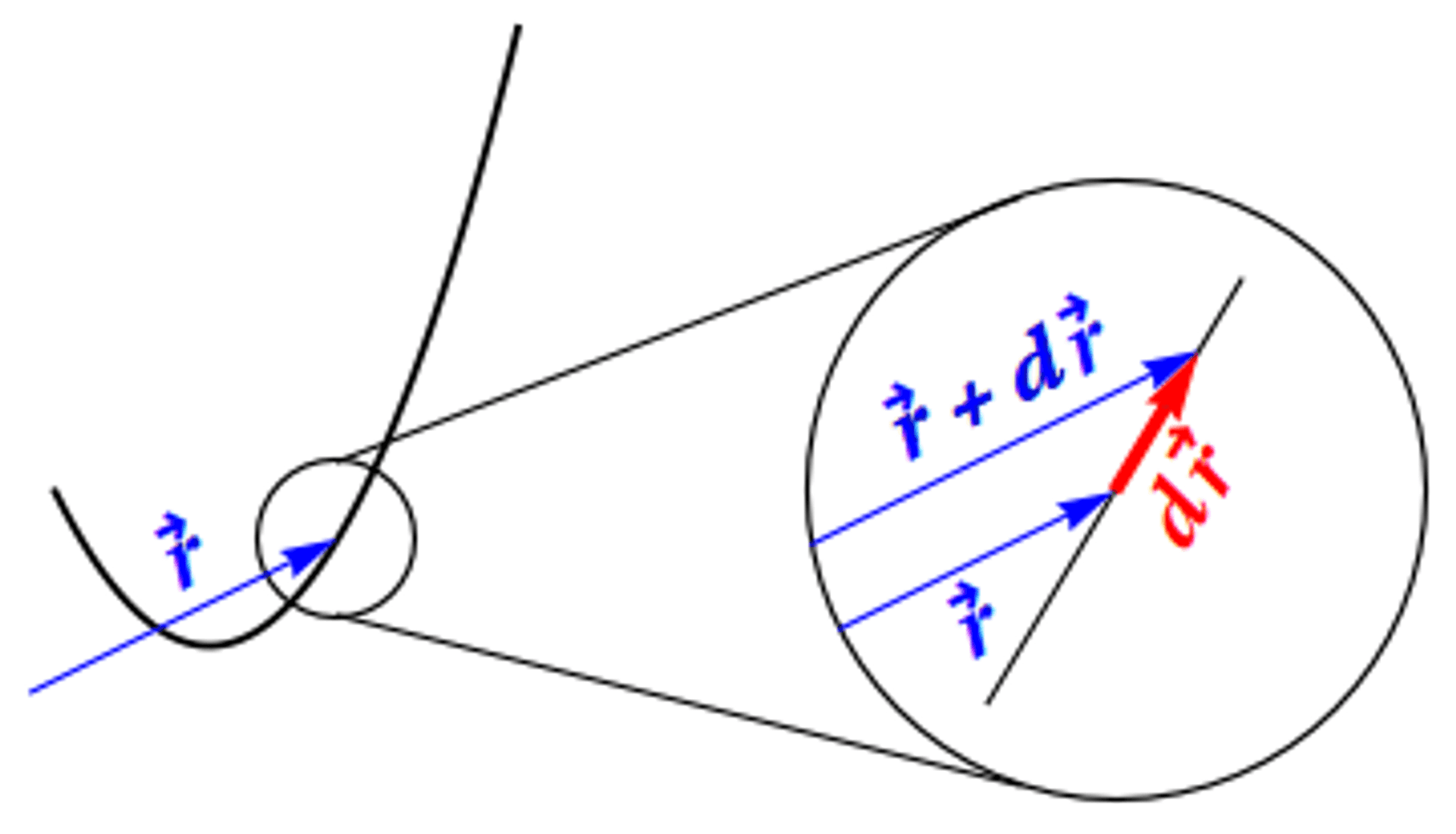
Figure 7 illustrates the infinitesimal displacement vector \(d\mathbf{r}\) along a curve, shown in an "infinite magnifying glass." The position vector \(\mathbf{r}=x\mathbf{\hat{x}}+y\mathbf{\hat{y}}+z\mathbf{\hat{z}}\) represents the location of the point \((x,y,z)\) in rectangular coordinates, originating from the origin. It is helpful to visualize the small change \(\Delta\mathbf{r}=\Delta x\mathbf{\hat{x}}+\Delta y\mathbf{\hat{y}}+\Delta z\mathbf{\hat{z}}\) in the position vector between nearby points. Taking a step further, we consider an infinitesimal change in position, denoted by \(d\mathbf{r}\), representing the vector between infinitesimally close points. Figure 7 provides a magnified view of the curve to illustrate this concept.

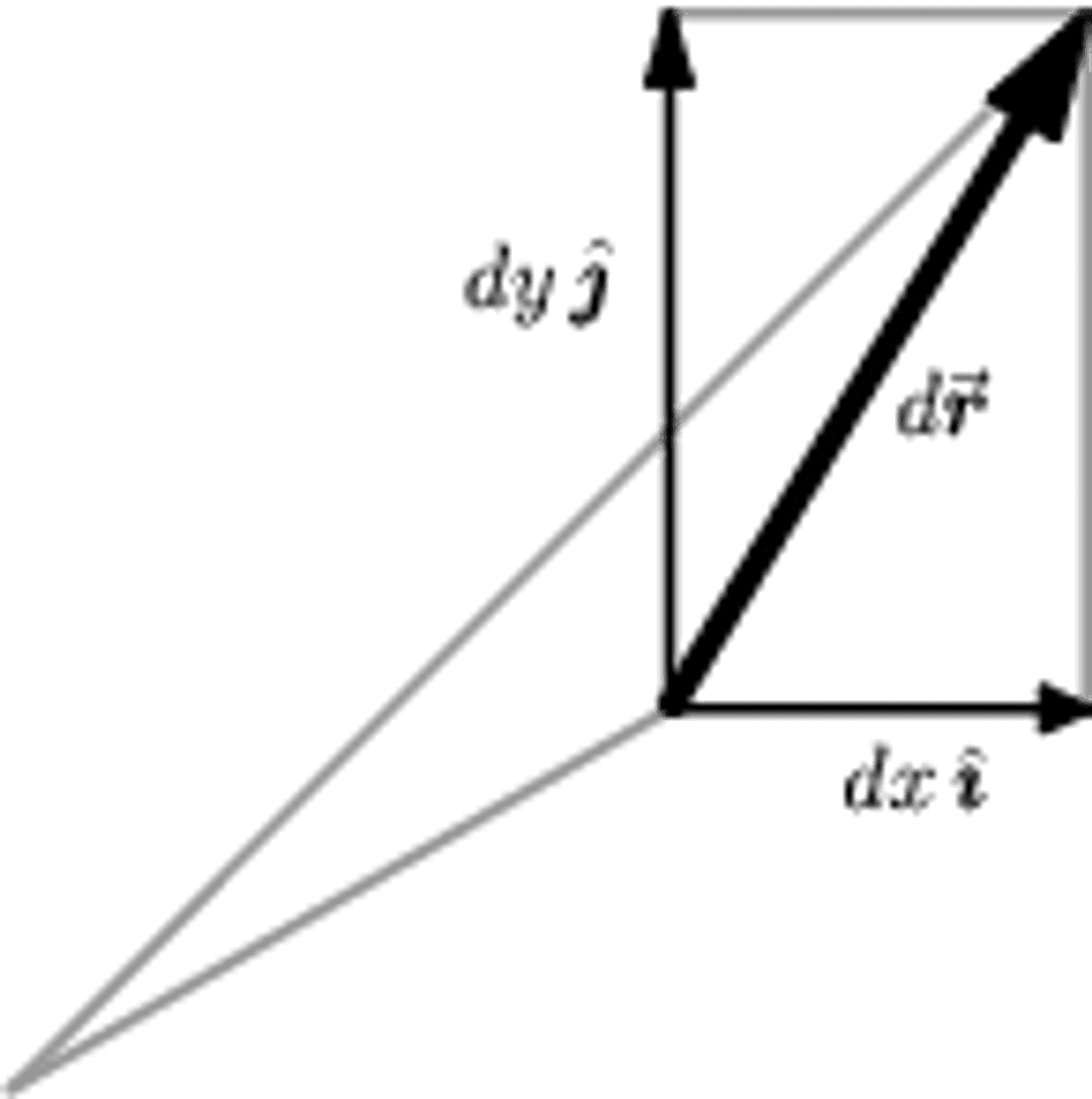
Figure 8a:

The rectangular components of the vector differential \(d\mathbf{r}\) in two dimensions.

Like any vector, \(d\mathbf{r}\) can be expanded with respect to \(\mathbf{\hat{x}}\), \(\mathbf{\hat{y}}\), \(\mathbf{\hat{z}}\); the components of \(d\mathbf{r}\) are just the infinitesimal changes \(dx\), \(dy\), \(dz\) in the \(x\), \(y\), and \(z\) directions, respectively. That is,

\[ d\mathbf{r} = dx\mathbf{\hat{x}} + dy\mathbf{\hat{y}} + dz\mathbf{\hat{z}} \label{drdef} \tag{1} \]

as shown in Figure 8a. The geometric notion of \(d\mathbf{r}\) as an infinitesimal vector displacement will be a unifying theme to help us visualize the geometry of all of vector calculus.

What is the infinitesimal distance \(ds\) between nearby points? It is simply the length of \(d\mathbf{r}\). We have

\[ ds = |d\mathbf{r}| = \sqrt{d\mathbf{r} \cdot d\mathbf{r}} = \sqrt{dx^2 + dy^2 + dz^2} \label{dsdef} \tag{2} \]

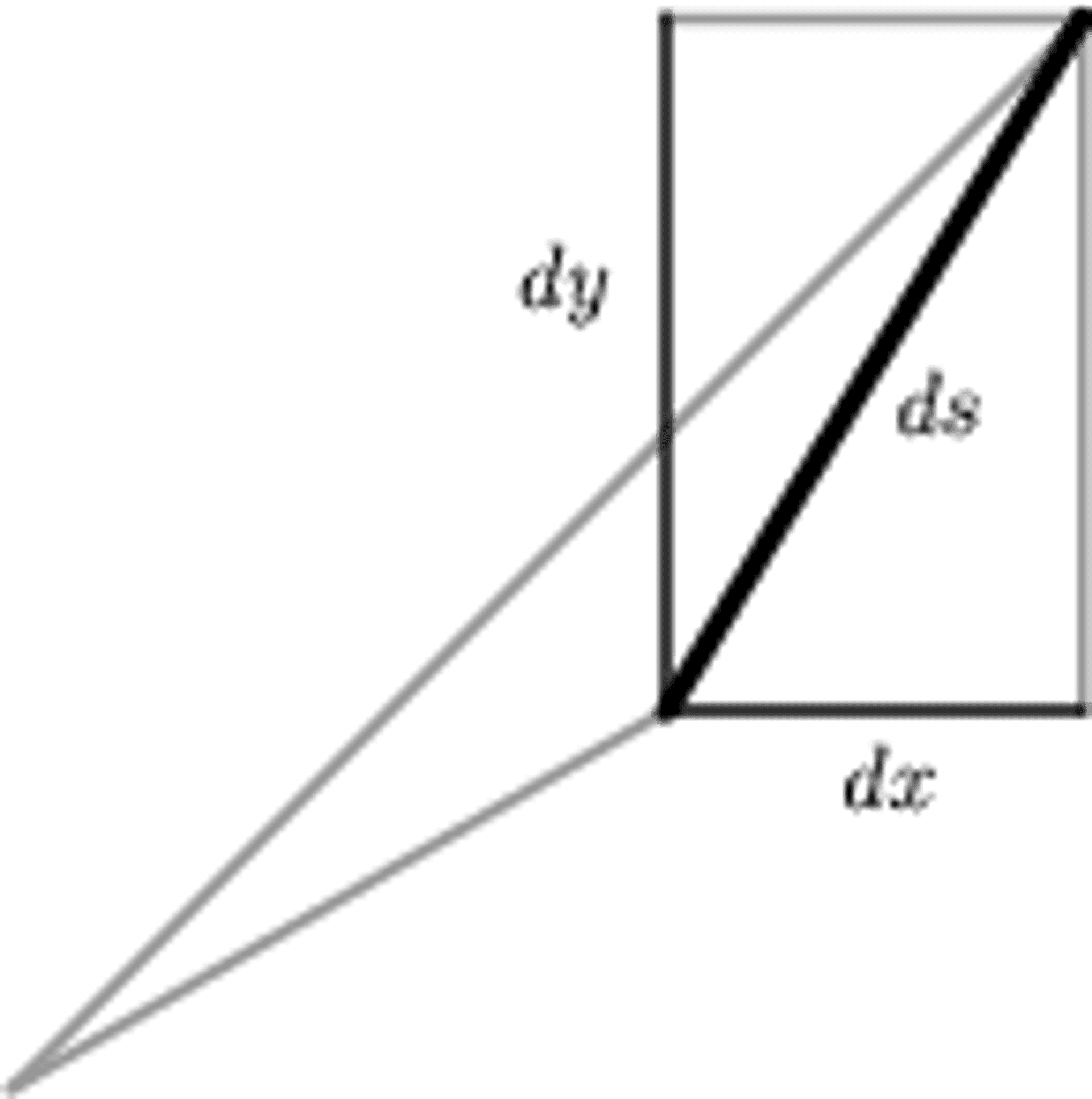
Figure 8b:

The infinitesimal version of the Pythagorean Theorem.

Squaring both sides of Equation \(\ref{dsdef}\) leads to

\[ ds^2 = |d\mathbf{r}|^2 = d\mathbf{r} \cdot d\mathbf{r} = dx^2 + dy^2 + dz^2 \label{ds1} \tag{3} \]

which is just the infinitesimal Pythagorean Theorem, the two-dimensional version of which is shown in Figure 8b.

When dealing with infinitesimals, we prefer to avoid second-order errors by anchoring all vectors to the same point.

vector differential in other coordinate systems

Staying strong with Tevian Dray and Corinne A. Manogue.

Figure 1a:

The infinitesimal vector version of the Pythagorean Theorem in rectangular coordinates.

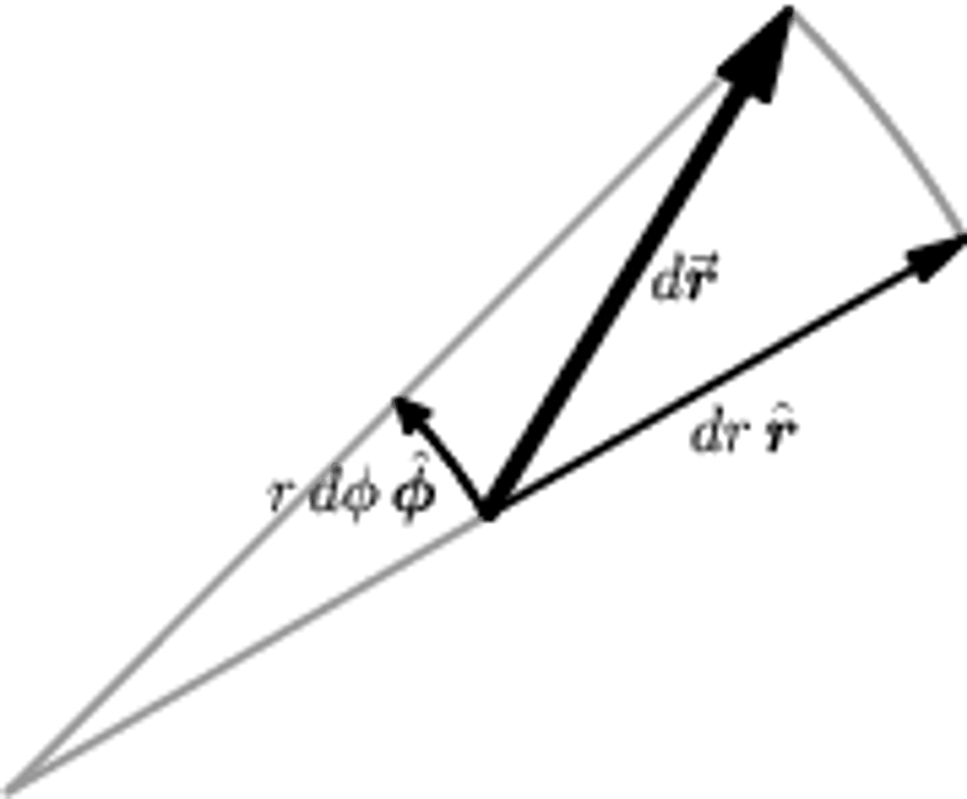
Figure 1b:

The infinitesimal vector version of the Pythagorean Theorem, in polar coordinates.

The Pythagorean Theorem in rectangular coordinates does not define \(d\vec{r}\) and \(ds\) in terms of component expressions (\(d\vec{r}\) being coordinate-independent). Instead, studying \(d\vec{r}\) in another coordinate system, such as polar coordinates (\(r, \phi\)), is useful. In polar coordinates, basis vectors \(\{\hat{r}, \hat{p}\}\) are used, with \(\hat{r}\) as the unit vector in the radial direction and \(\hat{p}\) as the unit vector in the direction of increasing \(\phi\).

By determining the lengths of the sides of the infinitesimal polar "rectangle" in Figure 1b, we find \(d\vec{r} = dr\,\hat{r} + r\,d\phi\,\hat{p}\). Note that the \(\hat{p}\) term includes a factor of \(r\), as \(d\phi\) alone is not a length. The length of an infinitesimal arc is \(r\,d\phi\). Using Equation (3) from the Vector Differential section, the length of \(d\vec{r}\) is given by \(ds^2 = dr^2 + r^2\,d\phi^2\), which is the infinitesimal Pythagorean Theorem in polar coordinates.

We adopt the polar angle \(\phi\) to align with the standard conventions for spherical coordinates used universally, except by American mathematicians.

It is possible to relate \(\hat{r}\) and \(\hat{p}\) to \(\hat{x}\) and \(\hat{y}\), but in most physical applications, an appropriate choice of coordinates eliminates the need for this step.

integration

Not too bad with Tevian Dray and Corinne A. Manogue at this point.

Integration involves dividing and adding smaller pieces, which is particularly useful for solving problems with multiple integrals. For example, when finding the mass of a straight wire with linear density \(\lambda\), we chop it into small pieces of length \(dx\). Each piece has a mass of \(\lambda dx\), and the total mass \(M\) is obtained by integrating \(\lambda(x)\) with respect to \(x\).

Similarly, in higher dimensions, such as for a rectangular plate with surface density \(\sigma\), we divide it into small rectangular pieces with area \(dA = dxdy\). The mass of each piece is \(\sigma dA\), and the total mass \(M\) is obtained by integrating \(\sigma(\mathbf{r})\) with respect to \(dA\).

In polar coordinates, if we have a circular plate with density \(\sigma = \sigma(r,\phi)\), we use polar pieces with area \(dA = rdrd\phi\). The total mass \(M\) is obtained by integrating \(\sigma(r,\phi)r\) with respect to \(r\) and \(\phi\).

While integration is commonly associated with finding antiderivatives and representing areas, it is important to understand the physical significance of infinitesimal mass \(\lambda dx\) and the choice of differential notation. Infinitesimally small pieces can be achieved by taking limits, and the notation involving differentials allows for a concise representation of this concept.

Note:

1. Differential notation emphasizes the ability to make pieces arbitrarily small and is shorthand for using Riemann sums with appropriate limits.
2. A single integral sign is used for adding rectangular pieces, while multiple integral signs are used for iterated single integrals.
3. The areas of infinitesimal rectangular and polar pieces are not comparable, and the choice of how to divide them does not affect the final result.

line integral

Oh, you thought I'd forget to mention Tevian Dray and Corinne A. Manogue.

There are many ways to describe a curve. Consider the following descriptions:

1. The unit circle
2. \(x^2 + y^2 = 1\)
3. \(y = 1 - \sqrt{1 - x^2}\)
4. \(r = 1\)
5. \(x = \cos\phi\), \(y = \sin\phi\)
6. \(\mathbf{r}(\phi) = \cos\phi\mathbf{\hat{x}} + \sin\phi\mathbf{\hat{y}}\)

If you want to add up something along a curve, you need to compute a line integral. Common examples include determining the length of a curve, the mass of a wire, or the amount of work done when moving an object along a specific path.

Let's consider the problem of finding the length of a quarter of a circle. In polar coordinates, a circle is represented by \(r = \text{constant}\), which implies \(dr = 0\). By substituting this fact into the expression for arc length in polar coordinates, we immediately obtain:

\[ds^2 = r^2d\phi^2 \quad (1)\]

and finally:

\[\int_C ds = \int_0^{\frac{\pi}{2}} r d\phi = \frac{\pi r^2}{2} \quad (2)\]

The calculation is not much harder in rectangular coordinates. You know that \(x = r\cos\phi\) and \(y = r\sin\phi\) with \(r = \text{constant}\), which gives \(dx = -r\sin\phi d\phi\) and \(dy = r\cos\phi d\phi\). By inserting this into (3) of The Vector Differential, \(ds^2 = |d\mathbf{r}|^2 = d\mathbf{r} \cdot d\mathbf{r} = dx^2 + dy^2 + dz^2 \), we arrive at (2) again.

But what if you didn't even remember how to parameterize a circle or how to use polar coordinates? Well, you still know that \(x^2 + y^2 = r^2 = \text{constant}\), which implies \(2xdx + 2ydy = 0\). Solving for \(dy\) and inserting this into (3) of The Vector Differential \(ds^2 = |d\mathbf{r}|^2 = d\mathbf{r} \cdot d\mathbf{r} = dx^2 + dy^2 + dz^2 \) yields:

\[ds^2 = \left(1 + \frac{x^2}{y^2}\right)dx^2 = \frac{r^2}{r^2 - x^2}dx^2 \quad (3)\]

This leads to the (improper!) integral:

\[\int_0^r \frac{dx}{\sqrt{1 - \frac{x^2}{r^2}}} \quad (4)\]

which can be easily computed using a trigonometric substitution or numerically, yielding the same answer.

scalar line integrals

Tevian Dray and Corinne A. Manogue stay strong as we move deeper in.

What if you want to determine the mass of a wire in the shape of the curve \(C\) if you know the density \(\lambda\)? The same procedure still works: chop and add. In this case, the length of a small piece of the wire is \(ds = |\mathbf{dr}|\), so its mass is \(\lambda ds\), and the integral becomes:

\[m = \int_C \lambda ds \quad (1)\]

which can also be written as:

\[m = \int_C \lambda(\mathbf{r}) |\mathbf{dr}| \quad (2)\]

which emphasizes both that \(\lambda\) is not constant and that \(ds\) is the magnitude of \(\mathbf{dr}\).

Another standard application of this type of line integral is to find the center of mass of a wire. This is done by averaging the values of the coordinates, weighted by the density \(\lambda\) as follows:

\[ \bar{x} = \frac{1}{m} \int_C x \lambda(\mathbf{r}) ds \quad (3) \]

with \(m\) as defined above. Similar formulas hold for \(\bar{y}\) and \(\bar{z}\); the center of mass is then the point \((\bar{x}, \bar{y}, \bar{z})\).

vector line integrals

Tevian Dray and Corinne A. Manogue do not have much to say about "Vector Line Integrals", but they give more context in other sections.

Consider now the problem of finding the work \(W\) done by a force \(\mathbf{F}\) in moving a particle along a curve \(C\). We begin with the relationship:

\[ \text{work} = \text{force} \times \text{distance} \quad (1) \]

Suppose you take a small step \(\mathbf{dr}\) along the curve. How much work was done? Since only the component along the curve matters, we need to take the dot product of \(\mathbf{F}\) with \(\mathbf{dr}\). Adding this up along the curve yields:

\[ W = \int_C \mathbf{F} \cdot \mathbf{dr} \quad (2) \]

So how do you evaluate such an integral?

An important special case of a line integral occurs when the curve \(C\) is closed, meaning it starts and ends at the same point. In this case, we write the integral in the form:

\[W = \oint_C \mathbf{F} \cdot d\mathbf{r} \quad (1)\]

and refer to it as the circulation of \(\mathbf{F}\) around \(C\). Unless otherwise specified, it is assumed that the curve is oriented in the counterclockwise direction. Reversing the orientation results in an overall minus sign, as with all vector line integrals.

This notation can also be used for scalar line integrals, such as finding the mass of a ring of wire, which could be written in the form:

\[M = \oint_C \lambda ds \quad (2)\]

Although in this case, the orientation doesn't matter. One way to remember this difference between vector and scalar integrals is to realize that \(ds = |d\mathbf{r}|\), and the magnitude of a vector does not depend on its direction.

path independence

I am grateful for Tevian Dray and Corinne A. Manogue.

RECALL: \(\int_a^b f'(x) \, dx = f(b) - f(a)\)

This is the Fundamental Theorem of Calculus, which states that the integral of a derivative is equal to the original function. We can also write it simply as: \(\int df = f\)

But recall the master formula of Gradients, which says: \(df = \nabla \cdot f \cdot d\mathbf{r}\)

Putting this all together, we arrive at the fundamental theorem for line integrals, which states that:

\[\int_C \nabla \cdot f \cdot d\mathbf{r} = f \, |_{A}^B\[

for any curve \(C\) starting at point A and ending at point B

Notice that the right-hand side does not depend on the curve \(C\).

There is some fine print here: the curve must lie in a connected region (one without holes) where \(\nabla \cdot f\) is defined everywhere. This is usually not a problem if \(f\) is differentiable everywhere, but there are important examples where this condition fails.

This behavior leads us to the notion of path independence. A line integral of the form \(\int_C \mathbf{F} \cdot d\mathbf{r}\) is said to be path independent if its value depends only on the endpoints A and B of the curve \(C\), and not on the specific curve connecting them. If a line integral is path independent, we can simply write:

\[\int_{A}^B \mathbf{F} \cdot d\mathbf{r}\]

If you know that a line integral is path independent, you can choose a different path (with the same endpoints) that simplifies the evaluation of the integral as much as possible!

conservative vector fields

Ok, Tevian Dray and Corinne A. Manogue really got into it for this section.

The fundamental theorem implies that vector fields of the form \(\mathbf{F} = \nabla f\) are special; the corresponding line integrals are always independent of path. One way to think of this is to imagine the level curves of \(f\); the change in \(f\) depends only on where you start and end, not on how you get there. These special vector fields have a name: A vector field \(\mathbf{F}\) is said to be conservative if there exists a potential function \(f\) such that \(\mathbf{F} = \nabla f\).

If \(\mathbf{F}\) is conservative, then \(\int_C \mathbf{F} \cdot d\mathbf{r}\) is independent of path; the converse is also true. But how do you know if a given vector field \(\mathbf{F}\) is conservative? That's the next lesson.

We describe here a variation of the usual procedure for determining whether a vector field is conservative and, if it is, for finding a potential function.

Figure 1a: Symbolic "tree diagram" for computing mixed partial derivatives with two variables.

Figure 1b: Symbolic "tree diagram" for computing mixed partial derivatives with three variables.

It is helpful to make a diagram of the structure underlying potential functions and conservative vector fields. For functions of two variables, this is shown in Figure 1a. The potential function \(f\) is shown at the top. Slanted lines represent derivatives of \(f\); derivatives with respect to \(x\) go to the left, while derivatives with respect to \(y\) go to the right. The second line thus gives the components of \(\nabla f\). The bottom line shows the mixed second derivatives, which can of course be computed in either order.

But what if we are not given \(f\)? Suppose we are given a vector field, such as \(\mathbf{F} = y\mathbf{i} + (x+2y)\mathbf{j}\) and need to determine whether it is conservative, that is, whether \(\mathbf{F}\) is the gradient of some potential function \(f\). This is the second line of the diagram! We could start by checking that the mixed derivatives agree. However, what we really want is the potential function; we should be moving up the diagram, not down. What happens if we simply integrate both components, as shown in Figure 2a? The potential function is clearly contained in the results of these two integrals; it is just a question of combining them correctly.

Furthermore, there is enough information here to determine whether \(\mathbf{F}\) is conservative in the first place; there is no need to check the derivatives. For example, had we been given the vector field \(\mathbf{H} = y\mathbf{i} + 2y\mathbf{j}\) and integrated its components, we would obtain Figure 2b. Simply by noticing that \(xy\), a function of two variables, only occurs once, we see that \(\mathbf{H}\) is not conservative.

Figure 2a: An inverted tree diagram for trying to find a potential function.

Figure 2b: Another inverted tree diagram for trying to find a potential function.

We describe this as a murder mystery. A crime has been committed by the unknown murderer \(f\); your job is to find the identity of \(f\) by interviewing the witnesses. Who are the witnesses? The components of the vector field. What do they tell you? Well, you have to integrate ("interrogate") them! Now for the fun part.

If two witnesses say they saw someone with red hair, that doesn't mean the suspect has two red hairs! So if you get the same clue more than once, you only count it once.

On the other hand, some clues require corroboration. These witnesses were situated in such a way that each could only look in one direction. Thus, one witness, the \(x\)-component, only sees terms involving \(x\), etc. If a clue contains more than one variable, it should have been seen by more than one witness! In fact, functions of \(n\) variables should occur precisely \(n\) times. In the case of the vector field \(\mathbf{H}\), the clue \(xy\) was only seen by one witness, not both; somebody is lying! In short, clues must be consistent.

Here is the Murder Mystery Method in a nutshell:

1. Integrate: Integrate the \(x\)-component with respect to \(x\), etc. 2. Check consistency: Functions of \(n\) variables must occur exactly \(n\) times. (If the consistency check fails, the vector field is not conservative.) 3. Combine clues: Use each clue once to determine the potential function.

The power of the murder mystery method is even more apparent in three dimensions. We encourage you to try to find a potential function for the vector field \(\mathbf{G} = yz\mathbf{i} + (xz+z)\mathbf{j} + (xy+y+2z)\mathbf{k}\) using this method. The underlying structure is shown in Figure 1b, where now \(y\) derivatives are shown going straight down, and \(z\) derivatives go to the right.

Consistency is traditionally checked by computing the last line of the appropriate diagram in Figures 1a and 1b. We reiterate that this is not necessary with the Murder Mystery Method. We will, however, return to these diagrams later when discussing the curl of a vector field.

1) Checking consistency may not be straightforward. Are \(-\cos^2 x \cos^2 y\) and \(\sin^2 x \cos^2 y\) the same? We have

which shows that the "xy" parts of these functions agree. (If this cannot be done, consistency fails.) But how do we count the remaining functions of 1 variable? Recall that the \(x\)-witness can only reliably provide clues involving \(x\)! If rewriting one or more functions this way generates a new such term, count it as usual. If instead, this generates a term involving the wrong variable(s), such as a clue provided by the \(x\)-witness that does not involve \(x\), discard it as unsubstantiated; this amounts to allowing the constant of integration to depend on the other variables. This procedure does not depend on the manner in which particular functions are rewritten, and such manipulations are not usually needed for typical classroom examples.

---

surface integrals

---

surface

Tevian Dray and Corinne A. Manogue say it like it is here.

Consider the following descriptions:

1. the unit sphere;
2. \(x^2+y^2+z^2=1;\)
3. \(r=1\) (where \(r\) is the spherical radial coordinate);
4. \(x=\sin\theta\cos\phi\), \(y=\sin\theta\sin\phi\), \(z=\cos\theta;\)
5. \(\mathbf{r}(\theta,\phi)=\sin\theta\cos\phi\mathbf{i}+\sin\theta\sin\phi\mathbf{j}+\cos\theta\mathbf{k};\)

all of which describe the same surface.

The simplest surfaces are those given by holding one of the coordinates constant. Thus, the xy-plane is given by \(z=0\). Its (surface) area element is \(dA=(dx)(dy)=(dr)(rd\phi)\), as can easily be seen by drawing the appropriate small rectangle. The surface of a cylinder is nearly as easy, as it is given by \(r=a\) in cylindrical coordinates, and drawing a small "rectangle" yields for the surface element:

Cylinder: \(dA=(a d\phi)(dz)=a d\phi dz\)

While a similar construction for the sphere given by \(r=a\) in spherical coordinates yields:

Sphere: \(dA=(a d\theta)(a\sin\theta d\phi)=a^2\sin\theta d\theta d\phi\)

The last expression can of course be used to compute the surface area of a sphere, which is:

\(\int_{\text{sphere}}dA=\int_{0}^{2\pi}\int_{0}^{\pi}a^2\sin\theta d\theta d\phi=4\pi a^2\)

What about more complicated surfaces?

The basic building block for surface integrals is the infinitesimal area \(dA\), obtained by chopping up the surface into small pieces. If the pieces are small parallelograms, then the area can be determined by taking the cross product of the sides!

Note: We write a single integral sign when talking about adding up "bits of area" (or "bits of volume"), reserving multiple integral signs for iterated single integrals. The notation \(\int\int dA\) is also common.

a bigger better cross product

Tevian Dray and Corinne A. Manogue did fine on this, but there's also a great stack exchange answer about cross products and antisymmetry.

The cross product is fundamentally a directed area. The magnitude of the cross product is defined to be the area of the parallelogram whose sides are the two vectors in the cross product.

In the figure above, if the horizontal vector is \(\mathbf{v}\) and the upward-pointing vector is \(\mathbf{w}\), then the height of the parallelogram is \(\left|\mathbf{w}\right|\sin\theta\), so its area is \(\left|\mathbf{v} \times \mathbf{w}\right| = \left|\mathbf{v}\right|\left|\mathbf{w}\right|\sin\theta\) \((1)\) which is therefore the magnitude of the cross product.

An immediate consequence of Equation \((1)\) is that, if two vectors are parallel, their cross product is zero, \(\mathbf{v} \parallel \mathbf{w} \implies \mathbf{v} \times \mathbf{w} = \mathbf{0}\) \((2)\) The direction of the cross product is given by the right-hand rule: Point the fingers of your right hand along the first vector (\(\mathbf{v}\)), and curl your fingers toward the second vector (\(\mathbf{w}\)). You may have to flip your hand over to make this work. Now stick out your thumb; that is the direction of \(\mathbf{v} \times \mathbf{w}\). In the example shown above, \(\mathbf{v} \times \mathbf{w}\) points out of the page. The right-hand rule implies that \(\mathbf{w} \times \mathbf{v} = -\mathbf{v} \times \mathbf{w}\) \((3)\) as you should verify for yourself by suitably positioning your hand. Thus, the cross product is not commutative. 1) Another important property of the cross product is that the cross product of a vector with itself is zero, \(\mathbf{v} \times \mathbf{v} = \mathbf{0}\) \((4)\) which follows from any of the preceding three equations.

In terms of the standard orthonormal basis, the geometric formula quickly yields

\[ \begin{align*} \hat{x} \times \hat{y} &= \hat{z} \\ \hat{y} \times \hat{z} &= \hat{x} \\ \hat{z} \times \hat{x} &= \hat{y} \end{align*} \]

This cyclic nature of the cross product can be emphasized by abbreviating this multiplication table as shown in the figure below. 2)Products in the direction of the arrow get a plus sign; products against the arrow get a minus sign.

Using an orthonormal basis such as \(\{\mathbf{x}, \mathbf{y}, \mathbf{z}\}\), the geometric formula reduces to the standard component form of the cross product. 3) If \(\mathbf{v} = v_x\mathbf{x} + v_y\mathbf{y} + v_z\mathbf{z}\) and \(\mathbf{w} = w_x\mathbf{x} + w_y\mathbf{y} + w_z\mathbf{z}\), then \(\mathbf{v} \times \mathbf{w} = (v_xw_y - v_yw_x)\mathbf{x} + (v_zw_x - v_xw_z)\mathbf{y} + (v_yw_z - v_zw_y)\mathbf{z}\) \((8)(9)\) which is often written as the symbolic determinant

\[\mathbf{v} \times \mathbf{w} = \begin{vmatrix} \mathbf{x} & \mathbf{y} & \mathbf{z} \\ v_x & v_y & v_z \\ w_x & w_y & w_z \end{vmatrix} \quad (10)\]

We encourage you to use \((10)\), rather than simply memorizing \((9)\). We also encourage you to compute the determinant as described below, rather than using minors; this tends to minimize sign errors. A \(3 \times 3\) determinant can be computed in the form

\[ \begin{vmatrix} a & b & c \\ d & e & f \\ g & h & i \end{vmatrix} = aei + bfg + cdh - ceg - bdi - afh \]

where one multiplies the terms along each diagonal line, subtracting the products obtained along lines going down to the left from those along lines going down to the right. While this method works only for \( (2 \times 2\) and \(3 \times 3\) determinants, it emphasizes the cyclic nature of the cross product.

Another important skill is knowing when not to use a determinant at all. For simple cross products, such as \((\mathbf{x} + 3\mathbf{y}) \times \mathbf{z}\), it is easier to use the multiplication table directly.

It is also worth pointing out that the multiplication table and the determinant method generalize naturally to any (right-handed) orthonormal basis; all that is needed is to replace the rectangular basis \(\{\mathbf{x}, \mathbf{y}, \mathbf{z}\}\) by the one being used (in the right order!). For example, in cylindrical coordinates, not only is

\[\mathbf{r} \times \boldsymbol{\phi} = \mathbf{z} \quad (11)\]

(and cyclic permutations), but cross products can be computed as

\[\mathbf{v} \times \mathbf{w} = \begin{vmatrix} \mathbf{r} & v_r & v_\phi & v_z \\ \mathbf{r} & w_r & w_\phi & w_z \\ \boldsymbol{\phi} & v_r & v_\phi & v_z \\ \boldsymbol{\phi} & w_r & w_\phi & w_z \\ \mathbf{z} & v_r & v_\phi & v_z \\ \mathbf{z} & w_r & w_\phi & w_z \end{vmatrix} \quad (12)\]

where of course \(\mathbf{v} = v_r\mathbf{r} + v_\phi\boldsymbol{\phi} + v_z\mathbf{z}\) and similarly for \(\mathbf{w}\).

A good problem emphasizing the geometry of the cross product is to find the area of the triangle formed by connecting the tips of the vectors \(\mathbf{x}\), \(\mathbf{y}\), \(\mathbf{z}\) (whose base is at the origin).

1) The cross product also fails to be associative, since for example \(\mathbf{x} \times (\mathbf{x} \times \mathbf{y}) = -\mathbf{y}\) but \((\mathbf{x} \times \mathbf{x}) \times \mathbf{y} = \mathbf{0}\).

2) This is really the multiplication table for the unit imaginary quaternions, a number system which generalizes the familiar complex numbers. Quaternions predate vector analysis, which borrowed the \(i\), \(j\), \(k\) notation for the rectangular basis vectors, which are often written as \(\mathbf{i}\), \(\mathbf{j}\), \(\mathbf{k}\). Here, we have adopted instead the more logical names \(\mathbf{x}\), \(\mathbf{y}\), \(\mathbf{z}\).

3) This argument uses the distributive property, which must be proved geometrically if one starts with \((1)\) and the right-hand rule. This is straightforward in two dimensions, but somewhat more difficult in three dimensions.

general surface

It is getting real with Tevian Dray and Corinne A. Manogue.

Since surfaces are two-dimensional, chopping up a surface is usually done by drawing two families of curves on the surface. Then you can compute \(d\mathbf{r}\) on each family and take the cross product, to get the vector surface element in the form \[ d\mathbf{S} = d\mathbf{r}_1 \times d\mathbf{r}_2 \label{Surface} \tag{1} \] In order to determine the area of the vector surface element, we need the magnitude of this expression, which is \[ dS = \lvert d\mathbf{r}_1\times d\mathbf{r}_2 \rvert \label{Scalar} \tag{2} \] and which is called the (scalar) surface element. This should remind you of the corresponding expression for line integrals, namely \(ds=\lvert d\mathbf{r} \rvert\).

We illustrate this technique by computing the surface element for the paraboloid given by \(z=x^2+y^2\), as shown in Figure 1, with the two families of curves corresponding to \(\{x=\text{const}\}\) and \(\{y=\text{const}\}\). We start with the basic formula for the vector differential \(d\mathbf{r}\), namely \[ d\mathbf{r} = dx\,\mathbf{\hat{x}} + dy\,\mathbf{\hat{y}} + dz\,\mathbf{\hat{z}} \] What do you know? The expression for \(z\) leads to \[ dz = 2x\,dx + 2y\,dy \] In rectangular coordinates, it is natural to consider infinitesimal displacements in the \(x\) and \(y\) directions. In the \(x\) direction, \(y\) is constant, so \(dy=0\), and we obtain \[ d\mathbf{r}_1 = dx\,\mathbf{\hat{x}} + 2x\,dx\,\mathbf{\hat{z}} = (\mathbf{\hat{x}} + 2x\,\mathbf{\hat{z}})\, dx \] Similarly, in the \(y\) direction, \(dx=0\), which leads to \[ d\mathbf{r}_2 = dy\,\mathbf{\hat{y}} + 2y\,dy\,\mathbf{\hat{z}} = (\mathbf{\hat{y}} + 2y\,\mathbf{\hat{z}})\, dy \] Putting this together, we obtain

for the vector surface element, andfor the scalar surface element.

This construction emphasizes that “area” is really a vector, whose direction is perpendicular to the surface, and whose magnitude is the area. Note that there are always two choices for the direction; choosing one determines the orientation of the surface.

When using \(\eqref{Surface}\) and \(\eqref{Scalar}\), it doesn't matter how you chop up the surface. It is of course possible to get the opposite orientation, for instance by interchanging the roles of \(d\mathbf{r}_1\) and \(d\mathbf{r}_2\). Rather than worrying too much about getting the “right” orientation from the beginning, it is usually simpler to check after you've calculated \(d\mathbf{S}\) whether the orientations you've got agrees with the requirements of the problem. If not, insert a minus sign.

Just as a curve is a 1-dimensional set of points, a surface is 2-dimensional. When computing line integrals, it was necessary to write everything in terms of a single parameter before integrating. Similarly, for surface integrals you must write everything, including the limits of integration, in terms of exactly two parameters before starting to integrate.

Finally, a word about notation. You will often see \(dS\) instead of \(dA\), and \(d\vec{S}\) instead of \(d\mathbf{S}\); most authors use \(dA\) in the \(xy\)-plane.

flux

Another slay from Tevian Dray and Corinne A. Manogue.

At any given point along a curve, there is a natural vector, namely the (unit) tangent vector \(\mathbf{T}\). Therefore, it is natural to add up the tangential component of a given vector field along a curve. When the vector field represents force, this integral represents the work done by the force along the curve. But there is no natural tangential direction at a point on a surface, or rather there are too many of them. The natural vector at a point on a surface is the (unit) normal vector \(\mathbf{n}\), so on a surface it is natural to add up the normal component of a given vector field; this integral is known as the flux of the vector field through the surface.

We already know that the vector surface element is given by

Since \(d\mathbf{r}_1\) and \(d\mathbf{r}_2\) are both tangent to the surface, \(d\mathbf{S}\) is perpendicular to the surface, and is therefore often writtenPutting this all together, the flux of a vector field \(\mathbf{F}\) through the surface is given by

We first consider a problem typical of those in calculus textbooks, namely finding the flux of the vector field \(\mathbf{F}=z\,\mathbf{\hat{z}}\) up through the part of the plane \(x+y+z=1\) lying in the first octant, as shown in Figure 1. We begin with the infinitesimal vector displacement in rectangular coordinates in 3 dimensions, namely

A natural choice of curves on this surface is given by setting \(y\) or \(x\) constant, so that \(dy=0\) or \(dx=0\), respectively. We thus obtain \begin{eqnarray} d\mathbf{r}_1 &=& dx\,\mathbf{\hat{x}} + dz\,\mathbf{\hat{z}} = (\mathbf{\hat{x}}-\mathbf{\hat{z}})\,dx \\ d\mathbf{r}_2 &=& dy\,\mathbf{\hat{y}} + dz\,\mathbf{\hat{z}} = (\mathbf{\hat{y}}-\mathbf{\hat{z}})\,dy \end{eqnarray} where we have used the equation of the plane to determine each expression in terms of a single parameter. The surface element is thus and the flux becomesThe limits were chosen by visualizing the projection of the surface into the \(xy\)-plane, which is a triangle bounded by the \(x\)-axis, the \(y\)-axis, and the line whose equation is \(x+y=1\). Note that this latter equation is obtained from the equation of the surface by using what we know, namely that \(z=0\).

Just as for line integrals, there is a rule of thumb which tells you when to stop using what you know to compute surface integrals: Don't start integrating until the integral is expressed in terms of two parameters, and the limits in terms of those parameters have been determined. Surfaces are two-dimensional!

Some readers will prefer to change the domain of integration in the second integral to be the projection of \(S\) into the \(xy\)-plane. We prefer to integrate over the actual surface whenever possible.

to symmetry or not to symmetry

Tevian Dray and Corinne A. Manogue pull out the double bind.

to symmetry

The electric field of a point charge \(q\) at the origin is given by

where \(\mathbf{\hat{r}}\) is the unit vector in the radial direction in spherical coordinates. Note that the first expression clearly indicates both the spherical symmetry of \(\mathbf{E}\) and its \(\frac{1}{r^2}\) fall-off behavior, while the second expression does neither.

It is easy to determine \(d\mathbf{S}\) on the sphere by inspection; we nevertheless go through the details of the differential approach for this case. We use “physicists' conventions” for spherical coordinates, so that \(\theta\) is the angle from the North Pole, and \(\phi\) the angle in the \(xy\)-plane. We use the obvious families of curves, namely the lines of latitude and longitude. Starting either from the general formula for \(d\mathbf{r}\) in spherical coordinates, namely

or directly using the geometry behind that formula, one quickly arrives at \begin{eqnarray} d\mathbf{r}_1 &=& r\,d\theta\,\mathbf{\hat{\theta}} \\ d\mathbf{r}_2 &=& r\sin\theta\,d\phi\,\mathbf{\hat{\phi}} \\ d\mathbf{S} &=& d\mathbf{r}_1 \times d\mathbf{r}_2 = r^2\sin\theta\,d\theta\,d\phi\,\mathbf{\hat{r}} \end{eqnarray} so thatYou may recognize this result as Gauss' Law, which says that the equation above gives the relationship between the total charge \(q\) inside any closed surface \(S\) and the flux of the electric field through the surface.

not to symmetry

The reader may have the feeling that two quite different languages are being spoken here. While the "use what you know" strategy may be somewhat unfamiliar, the basic idea should not be. On the other hand highly symmetric examples will be quite unfamiliar to most mathematicians, due to their use of adapted basis vectors such as \(\mathbf{\hat{r}}\). Mastering these examples helps develop experience looking for symmetry and making geometric arguments. At the same time, not all problems have symmetry!

We argue, however, that the approach being presented here is much more flexible than may appear at first sight. We demonstrate this flexibility by integrating over a paraboloid, the classic example found in calculus textbooks.

We compute the flux of the axially symmetric vector field \(\mathbf{F} = r\,\mathbf{\hat{r}} = x\,\mathbf{\hat{x}} + y\,\mathbf{\hat{y}}\) "outwards" through the part of the paraboloid \(z=r^2\) lying below the plane \(z=4\). The first thing we need is the formula for \(d\mathbf{r}\) in cylindrical coordinates, which is a straightforward generalization in polar coordinates, namely

spheres

Tevian Dray and Corinne A. Manogue have done it again.

Surprisingly, it often turns out to be simpler to solve problems involving spheres by working in cylindrical coordinates. We indicate here one of the reasons for this.

The equation of a sphere of radius \(a\) in cylindrical coordinates is 1)

so thatProceeding as for the paraboloid, we take \begin{align} d\mathbf{r}_1 &= r\,d\phi\,\mathbf{\hat{\phi}} \\ d\mathbf{r}_2 &= dr\,\mathbf{\hat{r}} + dz\,\mathbf{\hat{z}} = \left(-\frac{z}{r}\,\mathbf{\hat{r}} + \mathbf{\hat{z}}\right) dz \label{drdz} \end{align} where we now view \(r\) as a function of \(z\). We therefore havewhich results finally inThe surface element of a sphere is therefore the same as that of the cylinder of the same radius! Among other things, this means that projecting the Earth outward onto a cylinder is an equal-area projection, which is useful for cartographers.

parametric

You guessed it: another great take from Tevian Dray and Corinne A. Manogue.

The traditional approach to curves and surfaces involves parameterization, which we have deliberately saved for last. Recall that a parametric curve can be written \( \vec{r} = \vec{r}(u) = x(u)\,\hat{x} + y(u)\,\hat{y} + z(u)\,\hat{z} \) together with an appropriate domain for the parameter \( u \). A parametric surface is similar, except there are now two parameters \( u \), \( v \) (and an appropriate domain): \( \vec{r} = \vec{r}(u,v) = x(u,v)\,\hat{x} + y(u,v)\,\hat{y} + z(u,v)\,\hat{z} \)

Here are some examples of parametric surfaces (without domains): \[ \begin{align*} \text{sphere}: \quad & \vec{r}(\theta,\phi) = a\sin\theta\cos\phi\,\hat{x} + a\sin\theta\sin\phi\,\hat{y} + a\cos\theta\,\hat{z} \\ \text{cylinder}: \quad & \vec{r}(\phi,z) = a\cos\phi\,\hat{x} + a\sin\phi\,\hat{y} + z\,\hat{z} \\ z=f(x,y): \quad & \vec{r}(x,y) = x\,\hat{x} + y\,\hat{y} + f(x,y)\,\hat{z} \\ z=f(r,\phi): \quad & \vec{r}(r,\phi) = r\cos\phi\,\hat{x} + r\sin\phi\,\hat{y} + f(r,\phi)\,\hat{z} \\ \text{surface of revolution}: \quad & \vec{r}(x,\phi) = x\,\hat{x} + f(x)\cos\phi\,\hat{y} + f(x)\sin\phi\,\hat{z} \\ \text{change of variables}: \quad & \vec{r}(u,v) = x(u,v)\,\hat{x} + y(u,v)\,\hat{y} \end{align*} \]

Recall further that for a parametric curve we have \( d\vec{r} = \frac{d\vec{r}}{du} \,du \). On a parametric surface it is natural to construct \( d\textbf{S} \) using curves of constant parameter. But along a curve with \( v=\text{constant} \), we have \( d\vec{r}_1 = \frac{\partial\vec{r}}{\partial u} \,du \) and similarly along a curve with \( u=\text{constant} \) we have \( d\vec{r}_2 = \frac{\partial\vec{r}}{\partial v} \,dv \). Thus, \[ d\textbf{S} = d\vec{r}_1\times d\vec{r}_2 = \left(\frac{\partial\vec{r}}{\partial u} \times \frac{\partial\vec{r}}{\partial v}\right) \,du\,dv \] and \[ dS = |d\textbf{S}| = \left| \frac{\partial\vec{r}}{\partial u} \times \frac{\partial\vec{r}}{\partial v} \right| \,du \, dv \] These formulas can be found in most calculus texts, and may help to relate our approach to the more traditional one.

However, expression (1) of § Surface Elements for \( d\textbf{S} \) makes no reference to the parameters! In fact, \( d\textbf{S} \) can be computed using any two (independent) infinitesimal displacements in the surface; no parameterization is needed! You will have to decide for yourself which approach you prefer. But real-world problems rarely come equipped with parameterizations, unlike those found in calculus texts. We reiterate that it is not always necessary to have an explicit parameterization in order to determine the surface element, as illustrated by our computation for the paraboloid in § Less Symmetric Surfaces.

Scalar Surface Integrals

It should never be doubted whether Tevian Dray and Corinne A. Manogue can succeed.

Consider again the example in § Flux, which involved the part of the plane \(x+y+z=1\) which lies in the first quadrant. Suppose you want to find the average height of this triangular region above the \(xy\)-plane. To do this, chop the surface into small pieces, each at height \(z=1-x-y\). In order to compute the average height, we need to find \[ \text{avg height} = \frac{1}{\text{area}} \int z \,dS \] where the total area of the surface can be found either as \[ \text{area} = \int dS \] or from simple geometry. So we need to determine \(dS\). But we already know \(d\mathbf{S}\) for this surface from (5) of § Flux! It is therefore straightforward to compute \[ dS = |d\mathbf{S}| = |\mathbf{n} \cdot d\mathbf{S}| = |\mathbf{n}| \,dS = \sqrt{3} \,dS \] and therefore \[ \text{avg height} = \frac{1}{\sqrt{3}/2} \int_0^1 \int_0^{1-x} (1-x-y) \sqrt{3} \,dy \,dx = \frac{1}{3} \]

Function Graphs

Yes, please, more insight from Tevian Dray and Corinne A. Manogue.

We can apply these techniques to surfaces which are the graphs of functions. Suppose \(z=f(x,y)\). We slice the surface using curves along which either \(y\) is constant or \(x\) is constant. Since \[dz = df = \frac{\partial f}{\partial x}\,dx + \frac{\partial f}{\partial y}\,dy\] we obtain \[ d\mathbf{r}_1 = dx\,\mathbf{\hat{x}} + dz\,\mathbf{\hat{z}} = \left(\mathbf{\hat{x}} + \frac{\partial f}{\partial x}\,\mathbf{\hat{z}}\right)dx \] \[ d\mathbf{r}_2 = dy\,\mathbf{\hat{y}} + dz\,\mathbf{\hat{z}} = \left(\mathbf{\hat{y}} + \frac{\partial f}{\partial y}\,\mathbf{\hat{z}}\right)dy \] so that \[ d\mathbf{S} = d\mathbf{r}_1\times d\mathbf{r}_2 = \left( -\frac{\partial f}{\partial x}\,\mathbf{\hat{x}} - \frac{\partial f}{\partial y}\,\mathbf{\hat{y}} + \mathbf{\hat{z}} \right) \,dx\,dy \]

Similarly, if a scalar surface integral is needed, we can compute \[ dS = |d\mathbf{S}| = \sqrt{1+\left(\frac{\partial f}{\partial x}\right)^2+\left(\frac{\partial f}{\partial y}\right)^2}\,dx\,dy \]

You can find these formulas for \(d\mathbf{S}\) and \(dS\) in most textbooks on vector calculus.

Triple Product

One might wonder whether Tevian Dray and Corinne A. Manogue have ever missed.

Just as a parallelogram is the region in the plane divned by 2 vectors, a parallelepiped is the region in space divned by 3 vectors. Each side of a parallelepiped is therefore a parallelogram.

What is the volume of a parallelepiped? The area of its base times its height. But the base of a parallelepiped is a parallelogram, and the area of a parallelogram is just the magnitude of the cross product of its vector sides. The height of a parallelepiped must be measured perpendicular to the base, which is the same direction (up to sign) as that of the cross product just computed. Thus, the height of a parallelepiped is just the projection of the remaining side onto the direction of the cross product, and projections are accomplished by taking a dot product. This construction is illustrated in Figure 1. Putting this all together, the (signed) volume \(V\) of a parallelepiped divned by the vectors \(\mathbf{u}\), \(\mathbf{v}\), \(\mathbf{w}\) is given by the (scalar) triple product \[ V = (\mathbf{u}\times\mathbf{v})\cdot\mathbf{w} \] which is positive if \(\{\mathbf{u},\mathbf{v},\mathbf{w}\}\) are right-handed, and negative otherwise.

The geometric argument used in the above construction shows that the volume, and hence the triple product, is independent (up to sign) of the order of the vectors used to define it. Taking signs into account, we have: \[ (\mathbf{u}\times\mathbf{v})\cdot\mathbf{w} = (\mathbf{v}\times\mathbf{w})\cdot\mathbf{u} = (\mathbf{w}\times\mathbf{u})\cdot\mathbf{v} \] with the other three orderings differing by a minus sign. The three orderings \(\{\mathbf{u},\mathbf{v},\mathbf{w}\}\), \(\{\mathbf{v},\mathbf{w},\mathbf{u}\}\), \(\{\mathbf{w},\mathbf{u},\mathbf{v}\}\) are called cyclic permutations of each other; if one is right-handed, they are all right-handed. Note also that \[ \mathbf{w}\cdot(\mathbf{u}\times\mathbf{v}) = (\mathbf{u}\times\mathbf{v})\cdot\mathbf{w} = (\mathbf{w}\times\mathbf{u})\cdot\ mathbf{v} \] so that it doesn't matter whether the dot product is at the beginning or at the end. The cyclic nature of the triple product is summarized symbolically in Figure 2: So long as you write down the vectors in the order indicated by the arrow, it doesn't matter where you start, nor does it matter which product is a dot product, and which is a cross product. Of course, the parentheses do matter — you must evaluate the cross product before evaluating the dot product.

Using a symbolic determinant to compute the cross product, one quickly sees that the triple product is given by \[ (\mathbf{v}\times\mathbf{w})\cdot\mathbf{u} = \left| \begin{matrix} u_x & u_y & u_z \\ v_x & v_y & v_z \\ w_x & w_y & w_z \end{matrix} \right| \] from which the cyclic nature of the triple product also follows immediately, using standard properties of the determinant.

Volume Integrals

Straight from the wonderful Tevian Dray and Corinne A. Manogue.

The basic building block for volume integrals is the infinitesimal volume, obtained by chopping up the volume into small "parallelepipeds". Our approach for surface integrals can be extended to volume integrals using the triple product. The volume element becomes \[ dV = (\mathbf{d\mathbf{r}_1}\times\mathbf{d\mathbf{r}_2})\cdot\mathbf{d\mathbf{r}_3} \] for the \(\mathbf{d\mathbf{r}}\)'s computed for (any!) 3 non-coplanar families of curves. 1) (The volume element is often written as \(dV\), but we prefer \(\mathbf{dV}\) to avoid confusion with the electrostatic potential \(V\).) Using the natural families of curves in spherical coordinates, we could take \[ \mathbf{d\mathbf{r}_1} = r \,d\theta \,\mathbf{\hat{\theta}} \] \[ \mathbf{d\mathbf{r}_2} = r \,\sin\theta \,d\phi \,\mathbf{\hat{\phi}} \] as before, and add \[ \mathbf{d\mathbf{r}_3} = dr \,\mathbf{\hat{r}} \] leading to \[ \mathbf{dV} = r^2 \sin\theta \,dr \,d\theta \,d\phi \] as expected. For any orthogonal coordinate system, this method is of course equivalent to visualizing a small coordinate box and multiplying the lengths of the three sides.

The triple product has a cyclic symmetry, but the orientation matters — the order must be chosen so that \(\mathbf{dV}\) is positive.

Change of Variables

Tevian Dray and Corinne A. Manogue: in theaters near you.

Change of Variables \(R E C A L L: d A=d x d y=\boldsymbol{r} d \boldsymbol{r} d \boldsymbol{\phi}\) is the product \((d \boldsymbol{d})(\boldsymbol{r} d \boldsymbol{d}) .1)\) dimensions, yi el ding \[d V=(d x)(d y)(d z)=(d r)(r d \phi)(d z)=(d r)(r d \theta)(r \sin \theta d \phi)\] in Cartesi an, cylindrical, and spherical coordinates respectively. But what do we do if the coordinates are not orthogonal? We start by revi ewing the 1 -dimensional case, which is just the method of substitution. \(R E C A L L=x(u) \quad \Rightarrow \quad \int f d x=\int f \frac{d x}{d u} d u\) When making such a substitution, of course, one must replace \(\boldsymbol{x}\) everywhere by \(\boldsymbol{u}\), so that both \(\boldsymbol{f}\) and the integration limits must be rewritten in terms of \(\boldsymbol{u}\). Consider now a change of variables in two dimensions \[x=x(u, v) \quad y=y(u, v)\] We can therefore write the position vector as \[\overrightarrow{\mathbf{r}}=\overrightarrow{\mathbf{r}}(u, v)=\varkappa(u, v) \hat{\mathbf{x}}+v(u, v) \hat{\mathrm{y}}\] But this is just a special case of a parametric surface! We already know how to find the surface element of such surfaces. First compute \[d \overrightarrow{\mathbf{A}}=\overrightarrow{\mathbb{R}}_1 \times \overrightarrow{\vec{R}_2}=\left(\frac{\partial \overrightarrow{\mathbf{r}}}{\partial u} \times \frac{\partial \overrightarrow{\mathbf{r}}}{\partial v}\right) d u d v\] and then take the magnitude of \(\mathbf{d} \mathbf{A}\) to obtain \(\boldsymbol{d} \mathbf{A}\). We have This determinant is important enough to have its own name; we define the Jacobian of the transformation from \(\boldsymbol{u}, \boldsymbol{v}\) to \(\boldsymbol{x}, \boldsymbol{y}\) to be 2) \[\frac{\partial(x, y)}{\partial(u, v)}=\left|\begin{array}{ll} \frac{\partial x}{\partial v} & \frac{\partial y}{\partial v} \\ \frac{\partial z}{\partial v} & \frac{\partial v}{\partial v} \end{array}\right|=\left|\begin{array}{ll} \frac{\partial z}{\partial u} & \frac{\partial z}{\partial v} \\ \frac{\partial y}{\partial u} & \frac{\partial v}{\partial v} \end{array}\right|\] Putting this all together, we obtain \[d A=\left|\frac{\partial(x, y)}{\partial(u, v)}\right| d u d v\] Note that there are two sets of vertical bars here - this expressi on contains the absolute value of the Jacobian, since areas are positive. Not surprisingly, when this procedure is applied to the polar coordinate transformation \[x=r \cos \phi \quad y=r \sin \phi\] we get (check this yourself!) \[\frac{\partial(x, y)}{\partial(r, \phi)}=r\] so that, as we already knew, \(\boldsymbol{d A}=\boldsymbol{r} \boldsymbol{d} \boldsymbol{r} \boldsymbol{d \phi}\). therefore have \[\iint_R f d x d y=\iint f\left|\frac{\partial(x, y)}{\partial(u, v)}\right| d u d v\] what you know to rewrite all occurrences of \(\boldsymbol{x}\) and \(\boldsymbol{y}\) in terms of \(\boldsymbol{u}\) and \(\boldsymbol{v}\). To change variables in a double integral, Rewrite \(\boldsymbol{d A}\) in terms of the new variables using the above formula Rewrite the function being integrated in terms of the new variables. Change the limits from the old variables \((\boldsymbol{R})\) to the new ones \((\boldsymbol{D})\). A similar formula holds for triple integrals. Given \(\boldsymbol{x}, \boldsymbol{y}, \boldsymbol{z}\) as functions of \(\boldsymbol{u}, \boldsymbol{v}, \boldsymbol{w}\), the corresponding infinitesimal box is a parallelepiped with sides The volume of such a parallelepiped is given by the triple product \[d V=\left|\left({\overrightarrow{I_1}}_1 \times \overrightarrow{\vec{m}_2}\right) \cdot d \overrightarrow{\vec{r}_3}\right| d u d v d w\] Defining the Jacobian for transformations of three variables to be we obtain \[d V=\left|\frac{\partial(x, y, z)}{\partial(u, v, w)}\right| d u d v d w\]

Knowing \(\boldsymbol{d} \boldsymbol{V}\) we can convert any integral using \[\iiint f d x d y d z=\iiint f\left|\frac{\partial(x, y, z)}{\partial(u, v, w)}\right| d u d v d w\] for appropriate regions \(\boldsymbol{V}\) and \(\boldsymbol{W}\) (and with \(\boldsymbol{f}\) rewritten along the lines above). The above method for double integrals adapts easily to triple integrals. not only \[d x d y=\left|\frac{\partial(x, y)}{\partial(u, v)}\right| d u d v\] but also \[d u d v=\left|\frac{\partial(u, v)}{\partial(x, y)}\right| d u d y\] (17) from which we can conclude that \[\frac{\partial(x, y)}{\partial(u, v)}=1 / \frac{\partial(u, v)}{\partial(x, y)}\] reciprocal! really mean that the corresponding integrals are equal. 2) Recall that the determinant of the transpose of a matrix is the same as the determinant of the matrix

---

vector derivatives

---

divergence

Tevian Dray and Corinne A. Manogue convey divergence in the way they know best.

Consider a small closed box, with sides parallel to the coordinate planes, as shown in Figure 1. What is the flux of \(\mathbf{E}\) out of the box?

Consider first the vertical contribution, namely the flux up through the top plus the flux down through the bottom. These two sides each have area element \(dA=dx\,dy\), but the outward normal vectors point in opposite directions, that is

\[ \mathbf{n}_{\text{up}} = \mathbf{k} \\ \mathbf{n}_{\text{down}} = -\mathbf{k} \]

So, we get

\[ \sum_{\text{top+bottom}} \mathbf{E} \cdot d\mathbf{A} = \mathbf{E}(z+dz) \cdot \mathbf{k} > dx\,dy - \mathbf{E}(z) \cdot\mathbf{k} > dx\,dy \]

\[ = \Bigl( E_z(z+dz) - E_z(z) \Bigr) > dx\,dy \]

\[ = \frac{E_z(z+dz) - E_z(z)}{dz} > dx\,dy\,dz \]

where we have multiplied and divided by \(dz\) to obtain the volume element \(dV=dx\,dy\,dz\) in the third step, and used the definition of the derivative in the final step.

Repeating this argument using the remaining pairs of faces, it follows that the total flux out of the box is \[ \text{total flux} = \sum_{\text{box}} \mathbf{E} \cdot d\mathbf{A} = \left( \frac{\partial E_x}{\partial x} + \frac{\partial E_y}{\partial y} + \frac{\partial E_z}{\partial z} \right) > dV \] Since the total flux is proportional to the volume of the box, it approaches zero as the box shrinks down to a point. The interesting quantity is therefore the ratio of the flux to volume; this ratio is called the divergence.

At any point \(P\), we therefore define the divergence of a vector field \(\mathbf{E}\), written \(\nabla \cdot \mathbf{E}\), to be the flux of \(\mathbf{E}\) per unit volume leaving a small box around \(P\). In other words, the divergence is the limit as the box collapses around \(P\) of the ratio of the flux of the vector field out of the box to the volume of the box. Thus, the divergence of \(\mathbf{E}\) at \(P\) is the flux per unit volume through a small box around \(P\), which is given in rectangular coordinates by \[ \nabla \cdot \mathbf{E} = \frac{\text{flux}}{\text{unit volume}} = \frac{\partial E_x}{\partial x} + \frac{\partial E_y}{\partial y} + \frac{\partial E_z}{\partial z} \]

You may have seen this formula before, but remember that it is merely the rectangular coordinate expression for the divergence of \(\mathbf{E}\); the divergence is defined geometrically as flux per unit volume. Similar computations can be used to determine expressions for the divergence in other coordinate systems. Because of the geometric nature of divergence, these expressions turn out to give the same value at any point in space.

The use of \(V\) for volume, and hence \(dV\) for the volume element, conflicts with the use of \(V\) to denote electrostatic potential. We nonetheless write \(dV\) for the volume element whenever the context is clear, and use \(d\tau\) instead only when necessary to avoid confusion.

the divergence theorem

Tevian Dray and Corinne A. Manogue take divergence to the next level.

The total flux of the electric field out through a small rectangular box is \[ \text{flux} = \sum_{\text{box}} \mathbf{E} \cdot d\mathbf{A} = \nabla \cdot \mathbf{E} / dV \]

But any closed region can be filled with such boxes, as shown in Figure 1a. Furthermore, the flux out of such a region is just the sum of the flux out of each of the smaller boxes, since the net flux through any common face will be zero (because adjacent boxes have opposite notions of "out of"), as indicated schematically in Figure 1b. Thus, the total flux out of any closed box is given by \[ \int_{\text{box}} \mathbf{E} \cdot d\mathbf{A} = \int_{\text{inside}} \nabla \cdot \mathbf{E} > > dV \]

This is the Divergence Theorem.

the divergence in curvilinear coordinates

Tevian Dray and Corinne A. Manogue cannot be stopped with this divergence.

The divergence is defined in terms of flux per unit volume. We used this geometric definition to derive an expression for \(\nabla \cdot \mathbf{E}\) in rectangular coordinates, namely \[ \nabla \cdot \mathbf{E} = \frac{\text{flux}}{\text{unit volume}} = \frac{\partial E_x}{\partial x} + \frac{\partial E_y}{\partial y} + \frac{\partial E_z}{\partial z} \]

Similar computations to those in rectangular coordinates can be done using boxes adapted to other coordinate systems. Not surprisingly, this introduces some additional factors of \(r\) (and \(\sin\theta\)). For instance, consider a radial vector field of the form \[ \mathbf{E} = E_r \hat{r} \] where \(\hat{r}\) is the unit vector in the radial direction. The electric field of a point charge would have this form. What is the flux of \(\mathbf{E}\) through a small box around an arbitrary point \(P\), whose sides are surfaces with one of the spherical coordinates held constant, as shown in Figure 1? Only the two sides which are parts of spheres contribute, and each such contribution takes the form \[ \mathbf{E} \cdot d\mathbf{A} = \pm E_r r^2 \sin\theta \, d\theta \, d\phi \] An argument similar to the one used in rectangular coordinates leads to \[ \mathbf{E} \cdot d\mathbf{A} = \frac{1}{r^2} \frac{\partial}{\partial r} \left(r^2 E_r\right) \sin\theta \, dr \, d\theta \, d\phi = \frac{1}{r^2} \frac{\partial}{\partial r} \left(r^2 E_r\right) \, dV \] where it is important to note that the factor of \(r^2\) must also be differentiated. It now finally follows that \[ \nabla \cdot \mathbf{E} = \frac{1}{r^2} \frac{\partial}{\partial r} \left(r^2 E_r\right) \]

This expression only gives the divergence of the very special vector field \(\mathbf{E}\) given above. The full expression for the divergence in spherical coordinates is obtained by performing a similar analysis of the flux of an arbitrary vector field \(\mathbf{F}\) through our small box.

curl

Tevian Dray and Corinne A. Manogue have gone beyond divergence.

Consider a small rectangular loop in the \(yz\)-plane, with sides parallel to the coordinate axes, as shown in Figure 1. What is the circulation of \(\mathbf{A}\) around this loop?

Consider first the horizontal edges, on each of which \(\mathrm{d}\mathbf{r}=dy\,\mathbf{\hat{y}}\) . However, when computing the circulation of \(\mathbf{A}\) around this loop, we traverse these two edges in opposite directions. In particular, when traversing the loop in the counterclockwise direction, \(dy<0\) on top and \(dy>0\) on the bottom. We would like to compare these two edges, but we have \[ dy_{\text{top}} = -dy_{\text{bot}} \] so we conventionally set \(dy=dy_{\text{bot}}\) , leading to \(dy_{\text{top}}=-dy\) . Thus,

\[ \begin{align*} \sum_{\text{top+bottom}} \mathbf{A} \cdot \mathrm{d}\mathbf{r} &= - \mathbf{A}(z+dz)\cdot\mathbf{\hat{y}}\,dy + \mathbf{A}(z)\cdot\mathbf{\hat{y}}\,dy \\ &= - \Bigl( A_y(z+dz) - A_y(z) \Bigr)\,dy \\ &= - \frac{A_y(z+dz) - A_y(z)}{dz}\,dy\,dz \\ &= - \frac{\partial A_y}{\partial z}\,dy\,dz \end{align*} \]

where we have multiplied and divided by \(dz\) to obtain the surface element \(dA=dy\,dz\) in the third step, and used the definition of the derivative in the final step.

Just as with the divergence, in making this argument we are assuming that \(\mathbf{A}\) doesn't change much in the \(x\) and \(y\) directions, while nonetheless caring about the change in the \(z\) direction. We are again subtracting the values at two points separated in the \(z\) direction, so we are canceling the zeroth order term in \(z\), and therefore need the next order term. This can be made precise using a multivariable Taylor series expansion.

Repeating this argument for the remaining two sides leads to

\[ \sum_{\text{sides}}\mathbf{A} \cdot \mathrm{d}\mathbf{r} = \mathbf{A}(y+dy)\cdot\mathbf{\hat{z}}\,dz - \mathbf{A}(y)\cdot\mathbf{\hat{z}}\,dz = \Bigl( A_z(y+dy) - A_z(y) \Bigr)\,dz = \frac{A_z(y+dy) - A_z(y)}{dy}\,dy\,dz = \frac{\partial A_z}{\partial y}\,dy\,dz \]

where care must be taken with the signs, which are different from those in the equation (1). Adding up both expressions, we obtain \[ \text{total \(yz\)-circulation} = \left( \frac{\partial A_z}{\partial y} - \frac{\partial A_y}{\partial z} \right) dx\,dy \] Since this is proportional to the area of the loop, it approaches zero as the loop shrinks down to a point. The interesting quantity is therefore the ratio of the circulation to area. This ratio is almost the curl, but not quite.

We could have oriented our loop any way we liked. We have a circulation for each orientation, which we can associate with the normal vector to the loop; curl is a vector quantity. Our loop has counterclockwise orientation of the loop as seen from the positive \(x\)-axis; we are computing the \(\mathbf{\hat{x}}\)-component of the curl.

Putting this all together, we define the \(\mathbf{\hat{x}}\)-component of the curl of a vector field \(\mathbf{A}\) to be \[ \text{curl}(\mathbf{A})\cdot\mathbf{\hat{x}} = \frac{\text{\(yz\)-circulation}}{\text{unit area}} = \frac{\partial A_z}{\partial y} - \frac{\partial A_y}{\partial z} \] The rectangular expression for the full curl now follows by cyclic symmetry, yielding \[ \text{curl}(\mathbf{A}) = \nabla\times\mathbf{A} = \left| \begin{matrix} \mathbf{\hat{x}} & \mathbf{\hat{y}} & \mathbf{\hat{z}} \\ \frac{\partial}{\partial x} & \frac{\partial}{\partial y} & \frac{\partial}{\partial z} \\ A_x & A_y & A_z \end{matrix} \right| \]

A similar argument using a finite box would require integrating around the loop, in which case the limits of integration would be equal and opposite for these two edges, leading to an equivalent minus sign when adding the integrals.

the geometry of curl

Tevian Dray and Corinne A. Manogue take curl beyond curl.

Put a paddlewheel into a moving body of water. Depending on the details of the flow, the paddlewheel might spin. Keeping its center fixed, change the orientation of the paddlewheel. There will be a preferred orientation, in which the paddlewheel spins the fastest.

We can investigate this situation for any vector field \(\mathbf{A}\). Pick a point \(P\) and compute the circulation of \(\mathbf{A}\) around a small loop centered at \(P\). Now change the orientation of the loop and do it again. The result depends on the size of the loop, so we divide by its area. There will be a preferred orientation in which the circulation per unit area will be a maximum. We define the curl of \(\mathbf{A}\), written \(\nabla\times\mathbf{A}\), to be the vector whose direction is given by the normal vector to the plane in which the circulation is greatest, and whose magnitude is that circulation divided by the area of the loop, in the limit as the loop shrinks to a point. This construction yields the curl of \(\mathbf{A}\) at \(P\), and we can repeat the process at any point; the curl of \(\mathbf{A}\) is a vector field.

What is the circulation per unit area at the point \(P\) in an arbitrary direction? That's just the projection of \(\nabla\times\mathbf{A}\) in the given direction. That is, \((\nabla\times\mathbf{A})\cdot\hat{\mathbf{u}}\) is the (limiting value of) the circulation per unit area around a loop whose normal vector is \(\hat{\mathbf{u}}\).

By choosing \(\hat{\mathbf{u}}\) to be \(\mathbf{\hat{x}}\), \(\mathbf{\hat{y}}\), and \(\mathbf{\hat{z}}\) in turn, we can therefore compute the components of \(\nabla\times\mathbf{A}\) in rectangular coordinates. For further details, see §  Curl .

formulas for div, grad, curl

Tevian Dray and Corinne A. Manogue enumerate the formulas here.

Rectangular Coordinates

\[ \begin{align*} d\mathbf{r} &= dx\,\mathbf{\hat{x}} + dy\,\mathbf{\hat{y}} + dz\,\mathbf{\hat{z}} \\ \mathbf{F} &= F_x\,\mathbf{\hat{x}} + F_y\,\mathbf{\hat{y}} + F_z\,\mathbf{\hat{z}} \end{align*} \]

\[ \begin{align*} \boldsymbol{\nabla} f &= \frac{\partial f}{\partial x}\,\mathbf{\hat{x}} + \frac{\partial f}{\partial y}\,\mathbf{\hat{y}} + \frac{\partial f}{\partial z}\,\mathbf{\hat{z}} \\ \boldsymbol{\nabla}\cdot\mathbf{F} &= \frac{\partial F_x}{\partial x} + \frac{\partial F_y}{\partial y} + \frac{\partial F_z}{\partial z} \\ \boldsymbol{\nabla}\times\mathbf{F} &= \left(\frac{\partial F_z}{\partial y}-\frac{\partial F_y}{\partial z}\right)\mathbf{\hat{x}} + \left(\frac{\partial F_x}{\partial z}-\frac{\partial F_z}{\partial x}\right)\mathbf{\hat{y}} + \left(\frac{\partial F_y}{\partial x}-\frac{\partial F_x}{\partial y}\right)\mathbf{\hat{z}} \end{align*} \]

Cylindrical Coordinates

\[ \begin{align*} d\mathbf{r} &= dr\,\mathbf{\hat{r}} + r\,d\phi\,\mathbf{\hat{\phi}} + dz\,\mathbf{\hat{z}} \\ \mathbf{F} &= F_r\,\mathbf{\hat{r}} + F_\phi\,\mathbf{\hat{\phi}} + F_z\,\mathbf{\hat{z}} \end{align*} \]

\[ \begin{align*} \boldsymbol{\nabla} f &= \frac{\partial f}{\partial r}\,\mathbf{\hat{r}} + \frac{1}{r}\frac{\partial f}{\partial \phi}\,\mathbf{\hat{\phi}} + \frac{\partial f}{\partial z}\,\mathbf{\hat{z}} \\ \boldsymbol{\nabla}\cdot\mathbf{F} &= \frac{1}{r}\frac{\partial}{\partial r}\left(rF_r\right) + \frac{1}{r}\frac{\partial F_\phi}{\partial \phi} + \frac{\partial F_z}{\partial z} \\ \boldsymbol{\nabla}\times\mathbf{F} &= \left(\frac{1}{r}\frac{\partial F_z}{\partial \phi} - \frac{\partial F_\phi}{\partial z}\right)\mathbf{\hat{r}} + \left(\frac{\partial F_r}{\partial z}-\frac{\partial F_z}{\partial r}\right)\mathbf{\hat{\phi}} + \frac{1}{r} \left(\frac{\partial}{\partial r}\left(rF_{\phi}\right) - \frac{\partial F_r}{\partial \phi}\right)\mathbf{\hat{z}} \end{align*} \]

Spherical Coordinates

\[ \begin{align*} d\mathbf{r} &= dr\,\mathbf{\hat{r}} + r\,d\theta\,\mathbf{\hat{\theta}} + r\,\sin\theta\,d\phi\,\mathbf{\hat{\phi}} \\ \mathbf{F} &= F_r\,\mathbf{\hat{r}} + F_\theta\,\mathbf{\hat{\theta}} + F_\phi\,\mathbf{\hat{\phi}} \end{align*} \]

\[ \begin{align*} \boldsymbol{\nabla} f &= \frac{\partial f}{\partial r}\,\mathbf{\hat{r}} + \frac{1}{r}\frac{\partial f}{\partial \theta}\,\mathbf{\hat{\theta}} + \frac{1}{r\sin\theta}\frac{\partial f}{\partial \phi}\,\mathbf{\hat{\phi}} \\ \boldsymbol{\nabla}\cdot\mathbf{F} &= \frac{1}{r^2}\frac{\partial}{\partial r}\left(r^2F_{r}\right) + \frac{1}{r\sin\theta}\frac{\partial}{\partial \theta}\left(\sin\theta F_{\theta}\right) + \frac{1}{r\sin\theta}\frac{\partial F_\phi}{\partial \phi} \\ \boldsymbol{\nabla}\times\mathbf{F} &= \frac{1}{r\sin\theta} \left(\frac{\partial}{\partial \theta}\left(\sin\theta F_{\phi}\right) - \frac{\partial F_\theta}{\partial \phi}\right)\mathbf{\hat{r}} + \frac{1}{r} \left(\frac{1}{\sin\theta} \frac{\partial F_r}{\partial \phi} - \frac{\partial}{\partial r}\left(rF_{\phi}\right)\right)\mathbf{\hat{\theta}} + \frac{1}{r} \left(\frac{\partial}{\partial r}\left(rF_{\theta}\right) - \frac{\partial F_r}{\partial \theta}\right)\mathbf{\hat{\phi}} \end{align*} \]

stokes' theorem

Tevian Dray and Corinne A. Manogue have brought it to the pinnacle.

The total circulation of the magnetic field around a small loop is given by \[ \begin{align*} \text{circulation} &= \sum_{\text{box}} \mathbf{B} \cdot d\mathbf{r} \\ &= (\boldsymbol{\nabla}\times\mathbf{B}) \cdot d\mathbf{A} \end{align*} \] where \(d\mathbf{A}=\mathbf{n}\,dA\), and \(\mathbf{n}\) is perpendicular to the (filled-in) loop.

But any surface can be filled with such loops, as shown in Figure 1a. Furthermore, the circulation around the edge of the surface is just the sum of the circulations around each of the smaller loops, since the circulation through any common side will be zero (because adjacent loops have opposite notions of "around"), as indicated schematically in Figure 1b. Thus, the total circulation around any loop is given by \[ \begin{align*} \oint\limits_{\text{loop}} \mathbf{B} \cdot d\mathbf{r} = \int_{\text{inside}} (\boldsymbol{\nabla}\times\mathbf{B}) \cdot d\mathbf{A} \end{align*} \] This is Stokes' Theorem.

There is no need for the "inside" of the loop to be planar. 1) Consider the surface shown in Figure 1c, which has the same boundary as the original loop. The circulation around interior loops cancels just as before, and Stokes' Theorem holds without modification. We like to describe such surfaces as "butterfly nets," whose rim is the original loop. Butterfly nets should be able to catch butterflies! In other words, they need an opening and a net. 2)

The orientations used in the two integrals in Stokes' Theorem must be compatible. This is easy if the loop lies in the \(xy\)-plane: Choose the circulation counterclockwise and the flux upward. More generally, for any loop which is more-or-less planar, the circulation should be counterclockwise when looking at the loop from "above", that is, from the direction in which the flux is being taken. (So you're really looking in the direction of negative flux.) An easy way to remember this is to take the flux up and the circulation counterclockwise when seen from above, with obvious modifications should the loop be sideways.

But what if the loop is not planar? What about a cylinder that is closed at one end? There are several strategies that can be used to obtain compatible orientations:

• Gears: Break up the surface into small loops, which can be thought of as small gears. Choose an orientation of the surface and look at the surface from "above". As the gears turn counterclockwise, the edge of the surface also turns; use that orientation to compute the circulation.
• Toothpicks: Think of the surface as a rubber sheet. Move the rubber sheet so that it is taut across the loop. Choose a compatible orientation using the "up" and "counterclockwise" rule. Now imagine putting toothpicks in the surface on the "up" side only, and move the rubber sheet back to the original position. The direction of the toothpicks gives you the compatible orientation of the surface.
• Left-Hand Rule: Walk around the edge of the surface, with your head up. That is, face in the direction \(\mathbf{T}\), with your head in the direction \(\mathbf{n}\) (where \(d\mathbf{r}=\mathbf{T}\,ds\) and \(d\mathbf{S}=\mathbf{n}\,\mathbf{dS}\)). In a compatible orientation, your left hand should point along the surface; if it doesn't, turn around (or stand on your head, but not both).

There is also no need for the loop itself to be planar.

visualizing divergence and curl

Tevian Dray and Corinne A. Manogue bring it back to Earth.

The Divergence Theorem says

which tells us thatso that the divergence measures how much a vector field "points out" of a box. Similarly, Stokes' Theorem sayswhich tells us thatso that the (orthogonal component of the) curl measures how much a vector field "goes around" a loop.

Can we use these ideas to investigate graphically the divergence and curl of a given vector field? Consider the two vector fields above. In each case, can you find the divergence? The \(k\)-component of the curl?

A natural place to start is at the origin. So draw a small box around the origin. 1) Is there circulation around the loop? Is there flux across the loop?

The figures above help us determine the divergence and curl at the origin , but not elsewhere. The divergence is a function, and the curl is a vector field, so both can vary from point to point. We therefore need to examine loops that are not at the origin. It is useful to adapt the shape of our loop to the vector field under consideration. Both of our vector fields are better adapted to polar coordinates than to rectangular, so we use polar boxes. Can you determine the divergence and the $k$-component of the curl using the loops below? Imagine trying to do the same thing with a rectangular loop or even a circular loop.

Finally, it is important to realize that not all vector fields that point away from the origin have divergence, and not all vector fields that go around the origin have curl. The two examples below demonstrate this important principle; they have no divergence or curl away from the origin. These examples represent solutions of Maxwell's equations for electromagnetism. The figure on the left describes the electric field of an infinite charged wire, and the figure on the right describes the magnetic field due to an infinite current-carrying wire (with current coming out of the page at the origin).

In two dimensions, both "boxes" are loops. In three dimensions, the oriented box used to measure circulation is still a loop, but the box used to measure flux is now an ordinary, 3-dimensional box.